

Now, after predicting the values in the test dataset, we need to compute the accuracy of the model to know where we stand. We will first combine the actual value and predicted values, and use the head function to visually see the difference between the actual and predicted values for a few of the rows. We will then convert the newly formed data into the data frame format. Based on a trial-and-error basis, we set a suitable threshold. In the following case, we consider the probabilities with a value greater than 0.7 as 1; otherwise, 0:
result<- cbind(testdata$life_expectancy_morethan_70, prediction)
result<- as.data.frame(result)
colnames(result) <- c("Actual","Prediction")
result$Predicted[result[2] > 0.7] <- 1
result$Predicted[result[2] <= 0.7] <- 0
result<-  result[ , -which(names(result) %in% c("Prediction"))]
head(result, 20)
The output is as follows:
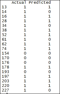
From the preceding output, we can visualize the difference between the Actual and...