Now, let's move on to actually defining the training models:

1. First, make an empty list, in which we will append the KNN model.
2. Enter the KNeighborsClassifier function and explore the number of neighbors.
3. Start with n_neighbors = 5, and play around with the variable a little, to see how it changes our results.

4. Next, we will add our models: the SVM and the SVC. We will evaluate each model, in turn.
5. The next step will be to get a results list and a names list, so that we can print out some of the information at the end.
6. We will then perform a for loop for each of the models defined previously, such as name or model in models.
7. We will also do a k-fold comparison, which will run each of these a couple of times, and then take the best results. The number of splits, or n_splits, defines how many times it runs.
8. Since we don't want a random state, we will go from the seed. Now, we will get our results. We will use the model_selection function that we imported previously, and the cross_val_score.
9. For each model, we'll provide training data to X_train, and then y_train.
10. We will also add the specification scoring, which was the accuracy that we added previously.
11. We will also append results, name, and we will print out a msg. We will then substitute some variables.
12. Finally, we will look at the mean results and the standard deviation.
13. A k-fold training will take place, which means that this will be run 10 times. We will receive the average result and the average accuracy for each of them. We will use a random seed of 8, so that it is consistent across different trials and runs. Now, press Shift + Enter. We can see the output in the following screenshot:

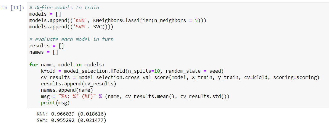
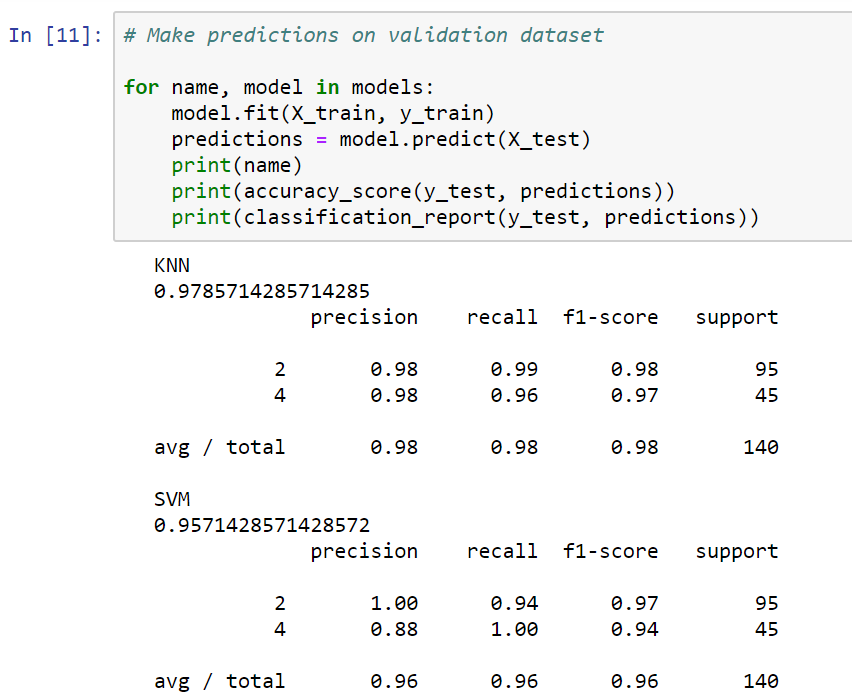
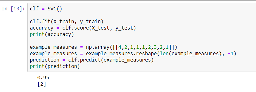
In this case, our KNN narrowly beats the SVC. We will now go back and make predictions on our validation set, because the numbers shown in the preceding screenshot just represent the accuracy of our training data. If we split up the datasets differently, we'll get the following results:

However, once again, it looks like we have pretty similar results, at least with regard to accuracy, on the training data between our KNN and our support vector classifier. The KNN tries to cluster the different data points into two groups: malignant and benign. The SVM, on the other hand, is looking for the optimal separating hyperplane that can separate these data points into malignant cells and benign cells.

In this section, we will make predictions on the validation dataset. So far, machine learning hasn't been very helpful, because it has told us information about the training data that we already know. Let's have a look at the following steps:

1. First, we will make predictions on the validation sets with the y_test and the X_test that we split out earlier.
2. We'll do another for loop in for name, and model in models.
3. Then, we will do the model.fit, and it will train it once again on the X and y training data. Since we want to make predictions, we're going to use the model to actually make a prediction about the X_test data.

4. Once the model has been trained, we're going to use it to make a prediction. It will print out the name, the accuracy score (based on a comparison of the y_test data with the predictions we made), and a classification_report, which will tell us information about the false positives and negatives that we found.
5. Now, press Shift + Enter. The following screenshot shows the preceding steps, and the output:

In the preceding screenshot, we can see that the KNN got a 98% accuracy rating in the validation set. The SVM achieved a result that was a little higher, at 95%.

The preceding screenshot also shows some other measures, such as precision, recall, and the f1-score. The precision is a measure of false positives. It is actually the ratio of correctly predicted positive observations to the total predicted positive observations. A high value for precision means that we don't have too many false positives. The SVM has a lower precision score than the KNN, meaning that it classified a few cases as malignant when they were actually benign. It is vital to minimize the chance of getting false positives in this case, especially because we don't want to mistakenly diagnose a patient with cancer.

The recall is a measure of false negatives. In our KNN, we actually have a few malignant cells that are getting through our KNN without being labeled. The f1-score column is a combination of the precision and recall scores.

We will now go back, to do another split and randomly sort our data again. In the following screenshot, we can see that our results have changed:

This time, we did much better on both the KNN and the SVM. We also got much higher precision scores from both, at 97%. This means that we probably only got one or two false positives for our KNN. We had no false negatives for our SVM, in this case.

We will now look into another example of predicting, once again based on the cell features:

1. First, we will make an SVC and get an accuracy score for it, based on our testing data.
2. Next, we will add an example. Type in np.array and pick whichever data points you want. We're going to need 10 of them. We also need to remember to see whether we get a malignant prediction.
3. We will then take example and add reshape to it. We will flip it around, so that we get a column vector.
4. We will then print our prediction and press Shift + Enter.

The following screenshot shows that we actually did get a malignant prediction:

In the preceding screenshot, we can see that we are 96% accurate, which is exactly what we were previously. By using the same model, we are actually able to predict whether a cell is malignant, based on its data.

When we run it again, we get the following results:

By changing the example from 1 to 10, the cells go from a malignant classification to a benign classification. When we change the values in the example from 4 to 5, we learn that 4 means that it is malignant. Thus, the difference between a 4 and a 5 is enough to switch our SVM from thinking it's a malignant cell to a benign cell.