A simple flow diagram of computation for a scientific application is depicted in the next diagram. The first step is to design a mathematical model for the problem under consideration. After the formulation of the mathematical model, the next step is to develop its algorithm. This algorithm is then implemented using a suitable programming language and an appropriate implementation framework. Selecting the programming language is a crucial decision that depends on the performance and processing requirements of the application. Another close decision is to finalize the framework to be used for the implementation. After deciding on the language and framework, the algorithm is implemented and sample simulations are performed. The results obtained from simulations are then analyzed for performance and correctness. If the result or performance of the implementation is not as per expectations, its causes should be determined. Then we need to go back to either reformulate the mathematical model, or redesign the algorithm or its implementation and again select the language and the framework.

A mathematical model is expressed by a set of suitable equations that describe most problems to the right extent of details. The algorithm represents the solution process in individual steps, and these will be implemented using a suitable programming language or scripting.

After implementation, there is an important step to perform—the simulation run of the implemented code. This involves designing the experimentation infrastructure, preparing or arranging the data/situation for simulation, preparing the scenario to simulate, and much more.

After completing a simulation run, result collection and its presentation are desired for the next step to analyze the results so as to test the validity of the simulation. If the results are not as they are expected, then this may require going back to one of the previous steps of the process to correct and repeat them. This situation is represented in the following figure in the form of dashed lines going back to some previous steps. If everything goes ahead perfectly, then the analysis will be the last step of the workflow, which is represented by double lines in this diagram:

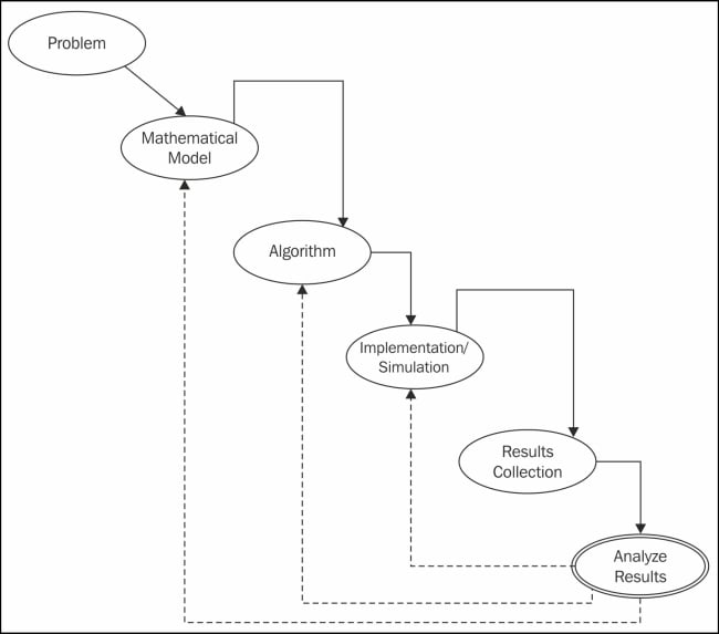
Various steps in a scientific computing workflow

The design and analysis of algorithms that solves any mathematical problem, specifically about science and engineering, is known as numerical analysis, and nowadays it is also called scientific computing. In scientific computing, the problems under consideration mainly deal with continuous values rather than discrete values. The latter are dealt with in other computer science problems. Generally saying, scientific computing solves problems that involve functions and equations with continuous variables, for example, time, distance, velocity, weight, height, size, temperature, density, pressure, stress, and much more.

Generally, problems of continuous mathematics have approximate solutions, as their exact solution is not always possible in a finite number of steps. Hence, these problems are solved using an iterative process that finally converges to an acceptable solution. The acceptable solution depends on the nature of the specific problem. Generally, the iterative process is not infinite, and after each iteration, the current solution gets closer to the desired solution for the purpose of simulation. Reviewing the accuracy of the solution and swift convergence to the solution form the gist of the scientific computing process.

There are well-established areas of science that use scientific computing to solve problems. They are as follows:

Recently, some emerging areas have also started harnessing the power of scientific computing. They include: