Sign In Start Free Trial
Account

Add to playlist

Create a Playlist

Modal Close icon
You need to login to use this feature.
  • Book Overview & Buying Mastering IPython 4.0
  • Table Of Contents Toc
Mastering IPython 4.0

Mastering IPython 4.0

By : Thomas Bitterman, Dipanjan Deb
3 (3)
close
close
Mastering IPython 4.0

Mastering IPython 4.0

3 (3)
By: Thomas Bitterman, Dipanjan Deb

Overview of this book

IPython is an interactive computational environment in which you can combine code execution, rich text, mathematics, plots, and rich media. This book will get IPython developers up to date with the latest advancements in IPython and dive deep into interactive computing with IPython. This an advanced guide on interactive and parallel computing with IPython will explore advanced visualizations and high-performance computing with IPython in detail. You will quickly brush up your knowledge of IPython kernels and wrapper kernels, then we'?ll move to advanced concepts such as testing, Sphinx, JS events, interactive work, and the ZMQ cluster. The book will cover topics such as IPython Console Lexer, advanced configuration, and third-party tools. By the end of this book, you will be able to use IPython for interactive and parallel computing in a high-performance computing environment.
Table of Contents (13 chapters)
close
close
6
6. Works Well with Others – IPython and Third-Party Tools
7
7. Seeing Is Believing– Visualization
12
Index

Going parallel

The previous sections are applicable to either serial or parallel computing. Even in the most parallelizable number crunching program, a great deal of serial code is written, so these observations are very applicable. After a certain point, however, parallel concerns come to dominate. We will start this section by introducing some terminology, before looking at a simple example.

Terminology

Wall-clock time is the amount of time that passes from the beginning of execution of a program to the end of its execution, as measured by looking at a clock on the wall. Wall-clock time is the measure people usually care about.

Cycle time is the time obtained by summing up the number of cycles taken by the program during its execution. For example, if a CPU is running at 1 MHz, each cycle takes 0.000001 seconds. So if it takes 2,500,000 cycles for a program to run, then it means the program took up 2.5 seconds of cycle time.

In a batch system with a single processor, the times are always the same. In a multitasking system, wall-clock time is often longer than cycle-time as the program may spend wall-clock time waiting to run without using any cycles.

With more than one processor, comparing the two times for an algorithm became more complicated. While not always true, many programs could be divided into pieces, such that running the program on two or more processors simultaneously reduced the wall-clock time, even if the cycle-time went up. Since wall-clock time is the important measure, for these algorithms, the answer was "Yes."

One can quantify this effect as follows:

Note

Given a particular algorithm A

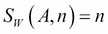
Call the wall-clock time for A when using n processors W(A, n).

Similarly, the cycle time for A using n processors is C(A, n).

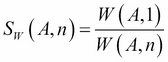
We can define the speedup of W(A, n) as Terminology

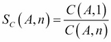
Similarly, we can define the speedup of C(A, n) as Terminology

In general, when using a batch system:

Note

For most algorithms, W(A, n) < C(A, n) when n > 1.

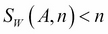
For most algorithms, Terminology when n > 1. For example, using two processors does not make the program run twice as fast. In general, adding more processors to run a program yields diminishing returns.

There are some algorithms for which Terminology. These are known as embarrassingly parallel algorithms. In this case, adding more processors results in linear speedup, which is where machines with many processors really shine.

In summary, the answer to the question, "Are more processors better?" is that it depends on the algorithm. Luckily for parallel computing, many algorithms show some amount of speedup and many important problems can be solved using these algorithms.

A parallel programming example

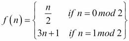
Consider the Collatz conjecture. Given the following function:

A parallel programming example

The conjecture is: for any positive integer, repeated application of f(n) will always reach the number 1. It is believed that the conjecture is true, but there is currently no proof. We are concerned with how long it takes to reach 1, that is, how many applications of f(n) are required for a given n. We would like to find the average for all n, 1 to 100.

The term for the sequence of numbers generated for any n is hailstone sequence. For example, the hailstone sequence for n = 6 is 6, 3, 10, 5, 16, 8, 4, 2, 1. We are interested in the average length of hailstone sequences.

A serial program

A regular (serial) Python program for computing the answer might look as follows:

def f(n):
    curr = n
    tmp = 1
    while curr != 1:
        tmp = tmp + 1
        if curr % 2 == 1:
            curr = 3 * curr + 1
        else:
            curr = curr/2
    return tmp

def main( ):
    sum = 0
    for i in range(1, 101):
        sum = sum + f(i)
    avg = sum / 100.0

Tip

Detailed steps to download the code bundle are mentioned in the Preface of this book. Please have a look.

The code bundle for the book is also hosted on GitHub at https://github.com/PacktPublishing/Mastering-IPython-4. We also have other code bundles from our rich catalog of books and videos available at https://github.com/PacktPublishing/. Check them out!

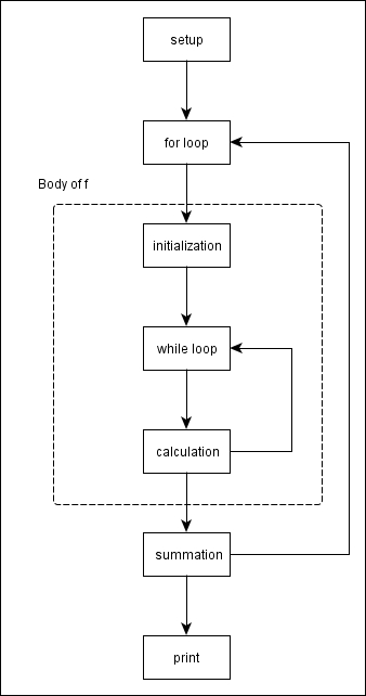
A schematic of the processing would look like this:

A serial program

Without going into too much detail, it is easy to see that the running time of the preceding program can be expressed as:

  • Setup (definition of f, initialization of sum, and so on)
  • Loop body (the sum of the amount of time to compute 100 hailstone sequences one at a time)
  • Teardown (calculate the average)

It is obvious that the running time of the program will be dominated by one of the loops. There is not much to be done about the while loop inside of f. Each iteration after the first depends on the result of a previous iteration. There is no way to, for example, do the tenth iteration without having already done the ninth, eighth, and so on.

The for loop inside of main has more potential for parallelization. In this case, every iteration is independent. That is:

  • Each iteration computes its own value, (f(i))
  • The computation of each f(i) does not depend on any other iteration
  • The values can easily be combined (via summation)

This algorithm can be converted to a parallel equivalent with a few extra commands. As they stand, these functions are pseudo-code—equivalent IPython functions will be described in later chapters:

  • getProcs(num): Returns a list of num processors
  • proc.setFun(fun, arg): Assigns a function fun with an argument arg to the proc processor
  • procs.executeAll( ): Executes fun on all processors in proc in parallel
  • proc.fetchValue( ): Returns the value computed on the proc processor when the calculation is complete

A parallel equivalent

With these additions, a parallel equivalent might look as follows:

def f(n):
    curr = n
    tmp = 1
    while curr != 1:
        tmp = tmp + 1
        if curr % 2 == 1:
            curr = 3 * curr + 1
        else:
            curr = curr/2
    return tmp

def main( ):
    sum = 0
    procs = getProcs(100)
    i = 1

    for proc in procs:
        proc.setFun(f, i)
        i = i + 1

    procs.executeAll( )

    for proc in procs:
        sum = sum + proc.fetchValue( )

    avg = sum / 100.0

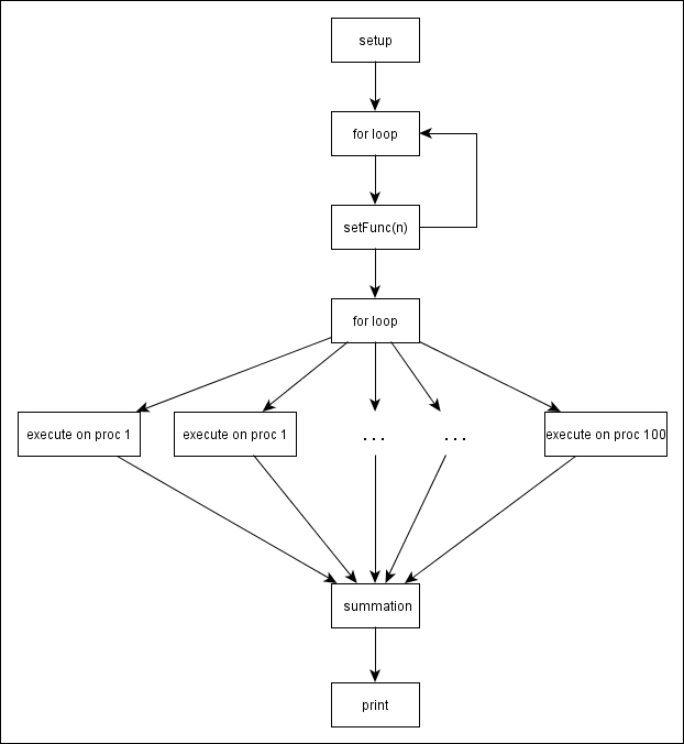
A schematic of the processing would look as follows:

A parallel equivalent

Discussion

While the parallel version is slightly longer (20 lines of code compared to 15), it is also faster, given enough processors. The intuitive reason is that the invocations of f are not queued up waiting for a single processor. With a single processor, the invocation of f(i) has to wait in line behind all the previous invocations of f(a) where 1 ≤ a < i, even though there is no dependency between them. The single processor is an unnecessary bottleneck. In this case, as no call to f depends on any other call, this algorithm is embarrassingly parallel.

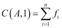
When a series of functions calls, (f1, f2, …, fn), is queued up for an algorithm A, it is easy to see that the cycle time required to complete all n function calls is:

Discussion

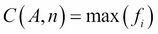
In the embarrassingly parallel case, the cycle time becomes (potentially) much smaller:

Discussion

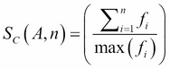
This results in a speedup (ignoring setup and teardown) of:

Discussion

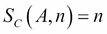
In the case where all fi use the same number of cycles, this simplifies to the following:

Discussion

Several issues important to parallel programming have been glossed over in the preceding discussion. These issues are important enough to have all of Chapter 3, Stepping Up to IPython for Parallel Computing, devoted to them.

CONTINUE READING
83
Tech Concepts
36
Programming languages
73
Tech Tools
Icon Unlimited access to the largest independent learning library in tech of over 8,000 expert-authored tech books and videos.
Icon Innovative learning tools, including AI book assistants, code context explainers, and text-to-speech.
Icon 50+ new titles added per month and exclusive early access to books as they are being written.
Mastering IPython 4.0
notes
bookmark Notes and Bookmarks search Search in title playlist Add to playlist download Download options font-size Font size

Change the font size

margin-width Margin width

Change margin width

day-mode Day/Sepia/Night Modes

Change background colour

Close icon Search
Country selected

Close icon Your notes and bookmarks

Confirmation

Modal Close icon
claim successful

Buy this book with your credits?

Modal Close icon
Are you sure you want to buy this book with one of your credits?
Close
YES, BUY

Submit Your Feedback

Modal Close icon
Modal Close icon
Modal Close icon