
We were talking about some of the most common NLP tools and preprocessing steps in the last chapter. This is the chapter where we will get to use most of the stuff we learnt in the previous chapters, and build one of the most sophisticated NLP applications. We will give you a generic approach about text classification and how you can build a text classifier from scratch with very few lines of code. We will give you a cheat sheet of all the classification algorithms in the context of text classification.
While we will talk about some of the most common text classification algorithms, this is just a brief introduction and to get to a detailed understanding and mathematical background, there are many online resources and books available that you can refer to. We will try to give you all you need to know to get you started with some working code snippets. Text classification is a great use case of NLP, but in this chapter, instead of using NLTK, we will use scikit-learn that has a wider range of classification algorithms and its library is much more memory efficient for text mining.
By the end of this chapter:
- You will learn and understand all text classification algorithms
- You will learn end-to-end pipeline to build a text classifier and how to implement it with scikit-learn and NLTK
The following is the scikit-learn cheat sheet for machine learning:
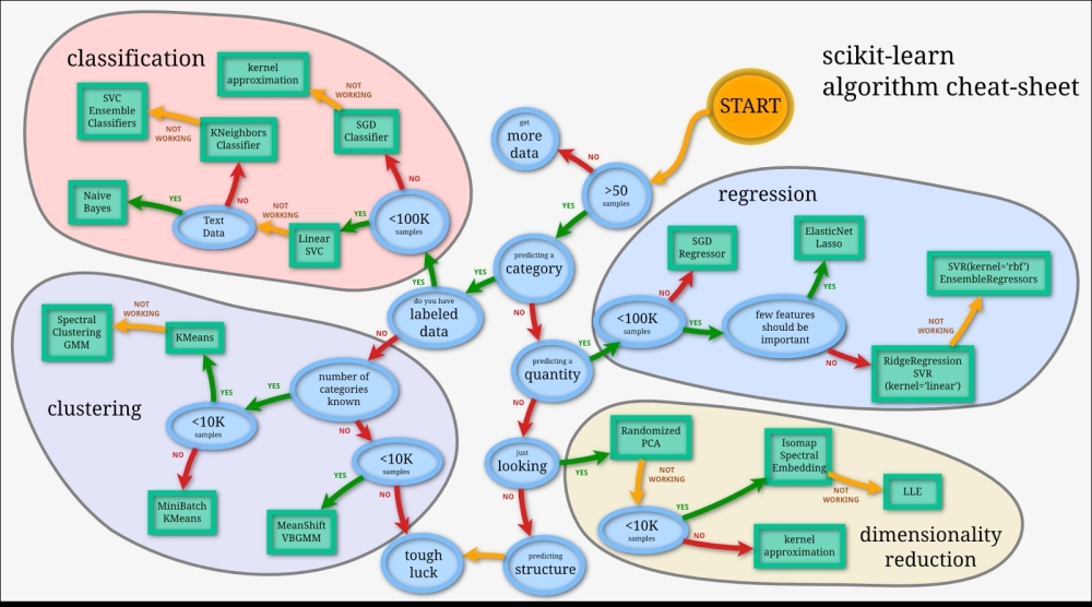
credit : scikit-learn
Now, as you travel along the process shown in the cheat sheet. We have a clear guideline about what kind of algorithm is required for which problem? When we should move from one classifier to another depending on the size of the tagged sample? It's a good place to start following this for building practical application, and in most cases this will work. We will focus mostly on text data while the scikit-learn can work with other types of data as well. We will explore text classification, text clustering, and topic detection in text (dimensionality reduction) with examples in this chapter and build some cool NLP applications. I will not go in to more detail about the concepts of machine learning, classification, and clustering in this chapter, as there are enough resources available on the Web for you. We will provide you with more details of all these concepts in the context of a text corpus. Still, let me give you a refresher.
There are two types of machine learning techniques—supervised learning and Unsupervised learning:
- Supervised learning: Based on some historic prelabeled samples, machines learn how to predict the future test sample, based on the following categories:
- Classification: This is used when we need to predict whether a test sample belongs to one of the classes. If there are only two classes, it's a binary classification problem; otherwise, it's a multiclass classification.
- Regression: This is used when we need to predict a continuous variable, such as a house price and stock index.
- Unsupervised learning: When we don't have any labeled data and we still need to predict the class label, this kind of learning is called unsupervised learning. When we need to group items based on similarity between items, this is called a clustering problem. While if we need to represent high-dimensional data in lower dimensions, this is more of a dimensionality reduction problem.
- Semi-supervised learning: This is a class of supervised learning tasks and techniques that also make use of unlabeled data for training. As the name suggests, it's more of a middle ground for supervised and unsupervised learning, where we use small amount of labeled data and large amount of unlabeled data to build a predictive machine learning model.
- Reinforcement learning: This is a form of machine learning where an agent can be programmed by a reward and punishment, without specifying how the task is to be achieved.
If you understood the different machine learning algorithms, I want you to guess what kind of machine learning problems the following are:
- You need to predict the values of weather for the next month
- Detection of a fraud in millions of transactions
- Google's priority inbox
- Amazon's recommendations
- Google news
- Self-driving cars
The simplest definition of text classification is that it is a classification of text based on the content of that text. Now, in general, all the machine learning methods and algorithms are written for numeric features/variables. One of the most important problems with text corpus is how to represent text as numeric features. There are different transformations prescribed in the literature. Let's start with one of the simplest and most widely used transformations.
Now, to understand the processes of text classification, let's take a real word problem of spams. In the world of WhatsApp and SMS, you get many spam messages. Let's start by solving this real problem of spam detection with the help of text classification. We will be using this running example across the chapter.
Here are a few real examples of SMS's that we asked people to manually tag for us:
SMS001 ['spam', 'Had your mobile 11 months or more? U R entitled to Update to the latest colour mobiles with camera for Free! Call The Mobile Update Co FREE on 08002986030']
SMS002 ['ham', "I'm gonna be home soon and i don't want to talk about this stuff anymore tonight, k? I've cried enough today."]
The first thing you want to do here is what we learnt in the last few chapters about data cleaning, tokenization, and stemming to get much cleaner content out of the SMS. I wrote a basic function to clean the text. Let's go over the following code:
>>>import nltk
>>>from nltk.corpus import stopwords
>>>from nltk.stem import WordNetLemmatizer
>>>import csv
>>>def preprocessing(text):
>>>    text = text.decode("utf8")
>>>    # tokenize into words
>>>    tokens = [word for sent in nltk.sent_tokenize(text) for word in nltk.word_tokenize(sent)]

>>>    # remove stopwords
>>>    stop = stopwords.words('english')
>>>    tokens = [token for token in tokens if token not in stop]

>>>    # remove words less than three letters
>>>    tokens = [word for word in tokens if len(word) >= 3]

>>>    # lower capitalization
>>>    tokens = [word.lower() for word in tokens]
>>>    # lemmatize
>>>    lmtzr = WordNetLemmatizer()
>>>    tokens = [lmtzr.lemmatize(word) for word in tokens]
>>>    preprocessed_text= ' '.join(tokens)
>>>    return preprocessed_text
We have talked about tokenization, lemmatization, and stop words in Chapter 3, Part of Speech Tagging. In the following code, I am just parsing the SMS file and cleaning the content to get cleaner text of the SMS. In the next few lines, I created two lists to get all the cleaned content of the SMS and class label. In ML (Machine learning) terms all the X and Y:
>>>smsdata = open('SMSSpamCollection') # check the structure of this file!
>>>smsdata_data = []
>>>sms_labels = []
>>>csv_reader = csv.reader(sms,delimiter='\t')
>>>for line in csv_reader:
>>>     # adding the sms_id
>>>    sms_labels.append( line[0])
>>>    # adding the cleaned text We are calling preprocessing method
>>>    sms_data.append(preprocessing(line[1]))
>>>sms.close()
Before moving any further we need to make sure we have scikit-learn installed on the system.
>>>import sklearn
Once we have the entire corpus in the form of lists, we need to perform some form of sampling. Typically, the way to sample the entire corpus in development train sets, dev-test sets, and test sets is similar to the sampling shown in the following figure.
The idea behind the whole exercise is to avoid overfitting. If we feed all the data points to the model, then the algorithm will learn from the entire corpus, but the real test of these algorithms is to perform on unseen data. In very simplistic terms, if we are using the entire data in the model learning process the classifier will perform very good on this data, but it will not be robust. The reason being, we have to tune it to perform the best on the given data, but it doesn't learn how to deal with unknown data.
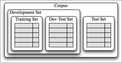
To solve this kind of a problem, the best way is to divide the entire corpus into two major sets. The development set and test set are kept away for the modeling exercise. We just use the dev set to build and tune the model. Once we are done with the entire modeling exercise, the results are projected based on the test set that we put aside. Now, if the model performs well on this set, we are sure that it's accurate and robust for any new data sample.
Sampling itself is a very complicated and well-researched stream in the machine learning community, and it's a remedy for many data skewness and overfitting issues. For simplicity, will use the basic sampling, where we just divide the corpus into a split of 70:30:
>>>trainset_size = int(round(len(sms_data)*0.70))
>>># i chose this threshold for 70:30 train and test split.
>>>print 'The training set size for this classifier is ' + str(trainset_size) + '\n'
>>>x_train = np.array([''.join(el) for el in sms_data[0:trainset_size]])
>>>y_train = np.array([el for el in sms_labels[0:trainset_size]])
>>>x_test = np.array([''.join(el) for el in sms_data[trainset_size+1:len(sms_data)]])
>>>y_test = np.array([el for el in sms_labels[trainset_size+1:len(sms_labels)]])or el in sms_labels[trainset_size+1:len(sms_labels)]])
>>>print x_train
>>>print y_train
- So what do you think will happen if we use the entire data as training data?
- What will happen when we have a very unbalanced sample?
Note
To understand more about the available sampling techniques, go through
http://scikit-learn.org/stable/modules/classes.html#module-sklearn.cross_validation.
Let's jump to one of the most important things, where we transform the entire text into a vector form. The form is referred to as the term-document matrix. If we have to create a term-document matrix for the given example, it will look somewhat like this:
|
TDM |
anymore |
call |
camera |
color |
cried |
enough |
entitled |
free |
gon |
had |
latest |
mobile |
|---|---|---|---|---|---|---|---|---|---|---|---|---|
|
SMS1 |
0 |
1 |
1 |
1 |
0 |
0 |
1 |
2 |
0 |
1 |
0 |
3 |
|
SMS2 |
1 |
0 |
0 |
0 |
1 |
1 |
0 |
0 |
1 |
0 |
0 |
0 |
The representation here of the text document is also known as the BOW (Bag of Word) representation. This is one of the most commonly used representation in text mining and other applications. Essentially, we are not considering any context between the words to generate this kind of representation.
To generate a similar term-document matrix in Python, we use scikit vectorizers:
>>>from sklearn.feature_extraction.text import CountVectorizer
>>>sms_exp=[ ]
>>>for line in sms_list:
>>>	sms_exp.append(preprocessing(line[1]))
>>>vectorizer = CountVectorizer(min_df=1)
>>>X_exp = vectorizer.fit_transform(sms_exp)
>>>print "||".join(vectorizer.get_feature_names())
>>>print X_exp.toarray()
array([[    1,    0,    1,    1,    1,    0,    0,    1,    2,    0,    1,    0,    1,    3,    1,    0,    0,    0,    1,    0,    0,    2,    0,    0], [    0,    1,    0,    0,    0,    1,    1,    0,    0,    1,    0,    1,    0,    0,    0,    1,    1,    1,    0,    1,    1,    0,    1,    1,    ]])
The count vectorizer is a good start, but there is an issue that you will face while using it: longer documents will have higher average count values than shorter documents, even though they might talk about the same topics.
Another refinement on top of tf is to downscale weights for words that occur in many documents in the corpus, and are therefore less informative than those that occur only in a smaller portion of the corpus.
This downscaling is called tf–idf (term frequency–inverse document frequency). Fortunately, scikit also provides a way to achieve the following:
>>>from sklearn.feature_extraction.text import TfidfVectorizer
>>>vectorizer = TfidfVectorizer(min_df=2, ngram_range=(1, 2),  stop_
words='english',  strip_accents='unicode',  norm='l2')
>>>X_train = vectorizer.fit_transform(x_train)
>>>X_test = vectorizer.transform(x_test)
We now have the text in a matrix format the same as we have in any machine learning exercise. Now, X_train and X_test can be used for classification using any machine learning algorithm. Let's talk about some of the most commonly used machine learning algorithms in context of text classification.
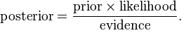
Let's build your first text classifier. Let's start with a Naive Bayes classifier. Naive Bayes relies on the Bayes algorithm and essentially, is a model of assigning a class label to the sample based on the conditional probability class given by features/attributes. Here we deal with frequencies/bernoulli to estimate prior and posterior probabilities.
The naive assumption here is that all features are independent of each other, which looks counter intuitive in the case of text. However, surprisingly, Naive Bayes performs quite well in most of the real-world use cases.
Another great thing about NB is that it's too simple and very easy to implement and score. We need to store the frequencies and calculate the probabilities. It's really fast in case of training as well as test (scoring). For all these reasons, in most of the cases of text classification, it serves as a benchmark.
Let's write some code to achieve this classifier:
>>>from sklearn.naive_bayes import MultinomialNB
>>>clf = MultinomialNB().fit(X_train, y_train)
>>>y_nb_predicted = clf.predict(X_test)
>>>print y_nb_predicted
>>>print ' \n confusion_matrix \n '
>>>cm = confusion_matrix(y_test, y_pred)
>>>print cm
>>>print '\n Here is the classification report:'
>>>print classification_report(y_test, y_nb_predicted)
confusion_matrix [[1205 5]
                  [26 156]]
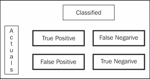
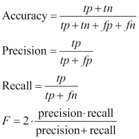
The way to read the confusion matrix is that from all the 1,392 samples in the test set, there were 1205 true positives and 156 true negative cases. However, we also predicted 5 false negatives and 26 false positives. There are different ways of measuring a typical binary classification.
We have given definitions of some of the most common measures used in classification measures:
Here is the classification report:
              Precision      recall      f1-score     support
ham           0.97           1.00        0.98         1210
spam          1.00           0.77        0.87         182
avg / total   0.97           0.97        0.97         1392
With the preceding definition, we can now understand the results clearly. So, effectively, all the preceding metrics look good, which means that our classifier is performing accurately, and is robust. I would highly recommend that you look into the module metrics for more options to analyze the results of the classifier. The most important and balanced metric is the f1 measure (which is nothing but the harmonic mean of precision and recall), which is used widely because it gives a better picture of the coverage and the quality of the classification algorithms. Accuracy intuitively tells us how many true samples have been covered from all the samples. Precision and recall both have significance, while precision talks about how many true positives it got and what else got covered, hand recall gives us details about how accurate we are from the pool of true positives and false negatives.
Note
For more information on various scikit classes visit the following link:
http://scikit-learn.org/stable/modules/classes.html#module-sklearn.metrics
The other more important process we follow to understand our model is to really look deep into the model by looking at the actual features that contribute to the positive and negative classes. I just wrote a very small snippet to generate the top n features and print them. Let's have a look at them:
>>>feature_names = vectorizer.get_feature_names()
>>>coefs = clf.coef_
>>>intercept = clf.intercept_
>>>coefs_with_fns = sorted(zip(clf.coef_[0], feature_names))
>>>n = 10
>>>top = zip(coefs_with_fns[:n], coefs_with_fns[:-(n + 1):-1])
>>>for (coef_1, fn_1), (coef_2, fn_2) in top:
>>>    print('\t%.4f\t%-15s\t\t%.4f\t%-15s' % (coef_1, fn_1, coef_2, fn_2))
-9.1602    10 den                 -6.0396    free               -9.1602    15                     -6.3487    txt                -9.1602    1hr                    -6.5067    text               -9.1602    1st ur                 -6.5393    claim              -9.1602    2go                    -6.5681    reply              -9.1602    2marrow                -6.5808    mobile             -9.1602    2morrow                -6.5858    stop               -9.1602    2mrw                   -6.6124    ur                 -9.1602    2nd innings            -6.6245    prize              -9.1602    2nd ur                 -6.7856    www
In the preceding code, I just read all the feature names from the vectorizer, got the coefficients related to the given feature, and then printed the first-10 features. If you want more features, just modify the value of n. If we look closely just at the features, we get a lot of information about the model as well as more suggestions about our feature selection and other parameters, such as preprocessing, unigrams/bigrams, stemming, tokenizations, and so on. For example, if you look at the top features of ham you can see that 2morrow, 2nd innings, and some of the digits are coming very significantly. We can see on the positive class (spam ) term "free" comes out a very significant term which is intuitive while many spam messages will be about some free offers and deal. Some of the other terms to note are prize, www, claim.
Decision trees are one of the oldest predictive modeling techniques, where for the given features and target, the algorithm tries to build a logic tree. There are multiple algorithms that exist for decision trees. One of the most famous and widely used algorithm is CART.
CART constructs binary trees using this feature, and constructs a threshold that yields the large amount of information from each node. Let's write the code to get a CART classifier:
>>>from sklearn import tree
>>>clf = tree.DecisionTreeClassifier().fit(X_train.toarray(), y_train)
>>>y_tree_predicted = clf.predict(X_test.toarray())
>>>print y_tree_predicted
>>>print ' \n Here is the classification report:'
>>>print classification_report(y_test, y_tree_predicted)
The only difference is in the input format of the training set. We need to modify the sparse matrix format to a NumPy array because the scikit tree module takes only a NumPy array.
Generally, trees are good when the number of features are very less. So, although our results look good here, people hardly use trees in text classification. On the other hand, trees have some really positive sides to them. It is still one the most intuitive algorithms and is very easy to explain and implement. There are many implementations of tree-based algorithms, such as ID3, C4.5, and C5. scikit-learn uses an optimized version of the CART algorithm.
Stochastic gradient descent (SGD) is a simple, yet very efficient approach that fits linear models. It is particularly useful when the number of samples (and the number of features) is very large. If you follow the cheat sheet, you will find SGD to be the one-stop solution for many text classification problems. Since it also takes care of regularization and provides different losses, it turns out to be a great choice when experimenting with linear models.
SGD, also known as Maximum entropy (MaxEnt), provides functionality to fit linear models for classification and regression using different (convex) loss functions and penalties. For example, with loss = log, fits a logistic regression model, while with loss = hinge, it fits a linear support vector machine (SVM).
An example of SGD is as follows:
>>>from sklearn.linear_model import SGDClassifier
>>>from sklearn.metrics import confusion_matrix
>>>clf = SGDClassifier(alpha=.0001, n_iter=50).fit(X_train, y_train)
>>>y_pred = clf.predict(X_test)
>>>print '\n Here is the classification report:'
>>>print classification_report(y_test, y_pred)
>>>print ' \n confusion_matrix \n '
>>>cm = confusion_matrix(y_test, y_pred)
>>>print cm
Here is the classification report:
             precision    recall    f1-score   support
ham          0.99         1.00      0.99       1210
spam         0.96         0.91      0.93       182
avg / total  0.98         0.98      0.98       1392
Most informative features:
    -1.0002    sir                    2.3815    ringtoneking
    -0.5239    bed                    2.0481    filthy
    -0.4763    said                   1.8576    service
    -0.4763    happy                  1.7623    story
    -0.4763    might                  1.6671    txt
    -0.4287    added                  1.5242    new
    -0.4287    list                   1.4765    ringtone
    -0.4287    morning                1.3813    reply
    -0.4287    always                 1.3337    message
    -0.4287    and                    1.2860    call
    -0.4287    plz                    1.2384    chat
    -0.3810    people                 1.1908    text
    -0.3810    actually               1.1908    real
    -0.3810    urgnt                  1.1431    video
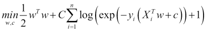
Logistic regression is a linear model for classification. It's also known in the literature as logit regression, maximum-entropy classification (MaxEnt), or the log-linear classifier. In this model, the probabilities describing the possible outcomes of a single trial are modeled using a logit function.
As an optimization problem, the L2 binary class' penalized logistic regression minimizes the following cost function:
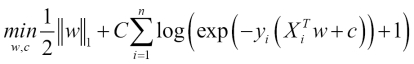
Similarly, L1 the binary class' regularized logistic regression solves the following optimization problem:
Support vector machines (SVM) is currently the-state-of-art algorithm in the field of machine learning.
SVM is a non-probabilistic classifier. SVM constructs a set of hyperplanes in an infinite-dimensional space, which can be used for classification, regression, or other tasks. Intuitively, a good separation is achieved by a hyperplane that has the largest distance to the nearest training data point of any class (the so-called functional margin), since in general, the larger the margin, the lower the size of classifier.
Let's build one of the most sophisticated supervised learning algorithms with scikit:
>>>from sklearn.svm import LinearSVC
>>>svm_classifier = LinearSVC().fit(X_train, y_train)
>>>y_svm_predicted = svm_classifier.predict(X_test)
>>>print '\n Here is the classification report:'
>>>print classification_report(y_test, y_svm_predicted)
>>>cm = confusion_matrix(y_test, y_pred)
>>>print cm
Here is the classification report for the same:
             precision    recall  f1-score   support
        ham       0.99      1.00      0.99      1210
       spam       0.97      0.90      0.93       182
avg / total       0.98      0.98      0.98      1392

confusion_matrix  [[1204    6] [  17  165]]
The most informative features:
    -0.9657    road                   2.3724    txt
    -0.7493    mail                   2.0720    claim
    -0.6701    morning                2.0451    service
    -0.6691    home                   2.0008    uk
    -0.6191    executive              1.7909    150p
    -0.5984    said                   1.7374    www
    -0.5978    lol                    1.6997    mobile
    -0.5876    kate                   1.6736    50
    -0.5754    got                    1.5882    ringtone
    -0.5642    darlin                 1.5629    video
    -0.5613    fullonsms              1.4816    tone
    -0.5613    fullonsms com          1.4237    prize
These are definitely the best results so far from all the supervised algorithms we have tried. Now with this, I will stop with supervised classifiers. There are millions of books available related to the different machine learning algorithms; even for individual algorithms, there are many books that are available for you. I would highly recommend you to have a deep understanding of any of the preceding algorithms before you use them for any of the real-world applications.
Naive Bayes
Let's build your first text classifier. Let's start with a Naive Bayes classifier. Naive Bayes relies on the Bayes algorithm and essentially, is a model of assigning a class label to the sample based on the conditional probability class given by features/attributes. Here we deal with frequencies/bernoulli to estimate prior and posterior probabilities.
The naive assumption here is that all features are independent of each other, which looks counter intuitive in the case of text. However, surprisingly, Naive Bayes performs quite well in most of the real-world use cases.
Another great thing about NB is that it's too simple and very easy to implement and score. We need to store the frequencies and calculate the probabilities. It's really fast in case of training as well as test (scoring). For all these reasons, in most of the cases of text classification, it serves as a benchmark.
Let's write some code to achieve this classifier:
>>>from sklearn.naive_bayes import MultinomialNB
>>>clf = MultinomialNB().fit(X_train, y_train)
>>>y_nb_predicted = clf.predict(X_test)
>>>print y_nb_predicted
>>>print ' \n confusion_matrix \n '
>>>cm = confusion_matrix(y_test, y_pred)
>>>print cm
>>>print '\n Here is the classification report:'
>>>print classification_report(y_test, y_nb_predicted)
confusion_matrix [[1205 5]
                  [26 156]]
The way to read the confusion matrix is that from all the 1,392 samples in the test set, there were 1205 true positives and 156 true negative cases. However, we also predicted 5 false negatives and 26 false positives. There are different ways of measuring a typical binary classification.
We have given definitions of some of the most common measures used in classification measures:
Here is the classification report:
              Precision      recall      f1-score     support
ham           0.97           1.00        0.98         1210
spam          1.00           0.77        0.87         182
avg / total   0.97           0.97        0.97         1392
With the preceding definition, we can now understand the results clearly. So, effectively, all the preceding metrics look good, which means that our classifier is performing accurately, and is robust. I would highly recommend that you look into the module metrics for more options to analyze the results of the classifier. The most important and balanced metric is the f1 measure (which is nothing but the harmonic mean of precision and recall), which is used widely because it gives a better picture of the coverage and the quality of the classification algorithms. Accuracy intuitively tells us how many true samples have been covered from all the samples. Precision and recall both have significance, while precision talks about how many true positives it got and what else got covered, hand recall gives us details about how accurate we are from the pool of true positives and false negatives.
Note
For more information on various scikit classes visit the following link:
http://scikit-learn.org/stable/modules/classes.html#module-sklearn.metrics
The other more important process we follow to understand our model is to really look deep into the model by looking at the actual features that contribute to the positive and negative classes. I just wrote a very small snippet to generate the top n features and print them. Let's have a look at them:
>>>feature_names = vectorizer.get_feature_names()
>>>coefs = clf.coef_
>>>intercept = clf.intercept_
>>>coefs_with_fns = sorted(zip(clf.coef_[0], feature_names))
>>>n = 10
>>>top = zip(coefs_with_fns[:n], coefs_with_fns[:-(n + 1):-1])
>>>for (coef_1, fn_1), (coef_2, fn_2) in top:
>>>    print('\t%.4f\t%-15s\t\t%.4f\t%-15s' % (coef_1, fn_1, coef_2, fn_2))
-9.1602    10 den                 -6.0396    free               -9.1602    15                     -6.3487    txt                -9.1602    1hr                    -6.5067    text               -9.1602    1st ur                 -6.5393    claim              -9.1602    2go                    -6.5681    reply              -9.1602    2marrow                -6.5808    mobile             -9.1602    2morrow                -6.5858    stop               -9.1602    2mrw                   -6.6124    ur                 -9.1602    2nd innings            -6.6245    prize              -9.1602    2nd ur                 -6.7856    www
In the preceding code, I just read all the feature names from the vectorizer, got the coefficients related to the given feature, and then printed the first-10 features. If you want more features, just modify the value of n. If we look closely just at the features, we get a lot of information about the model as well as more suggestions about our feature selection and other parameters, such as preprocessing, unigrams/bigrams, stemming, tokenizations, and so on. For example, if you look at the top features of ham you can see that 2morrow, 2nd innings, and some of the digits are coming very significantly. We can see on the positive class (spam ) term "free" comes out a very significant term which is intuitive while many spam messages will be about some free offers and deal. Some of the other terms to note are prize, www, claim.
Decision trees are one of the oldest predictive modeling techniques, where for the given features and target, the algorithm tries to build a logic tree. There are multiple algorithms that exist for decision trees. One of the most famous and widely used algorithm is CART.
CART constructs binary trees using this feature, and constructs a threshold that yields the large amount of information from each node. Let's write the code to get a CART classifier:
>>>from sklearn import tree
>>>clf = tree.DecisionTreeClassifier().fit(X_train.toarray(), y_train)
>>>y_tree_predicted = clf.predict(X_test.toarray())
>>>print y_tree_predicted
>>>print ' \n Here is the classification report:'
>>>print classification_report(y_test, y_tree_predicted)
The only difference is in the input format of the training set. We need to modify the sparse matrix format to a NumPy array because the scikit tree module takes only a NumPy array.
Generally, trees are good when the number of features are very less. So, although our results look good here, people hardly use trees in text classification. On the other hand, trees have some really positive sides to them. It is still one the most intuitive algorithms and is very easy to explain and implement. There are many implementations of tree-based algorithms, such as ID3, C4.5, and C5. scikit-learn uses an optimized version of the CART algorithm.
Stochastic gradient descent (SGD) is a simple, yet very efficient approach that fits linear models. It is particularly useful when the number of samples (and the number of features) is very large. If you follow the cheat sheet, you will find SGD to be the one-stop solution for many text classification problems. Since it also takes care of regularization and provides different losses, it turns out to be a great choice when experimenting with linear models.
SGD, also known as Maximum entropy (MaxEnt), provides functionality to fit linear models for classification and regression using different (convex) loss functions and penalties. For example, with loss = log, fits a logistic regression model, while with loss = hinge, it fits a linear support vector machine (SVM).
An example of SGD is as follows:
>>>from sklearn.linear_model import SGDClassifier
>>>from sklearn.metrics import confusion_matrix
>>>clf = SGDClassifier(alpha=.0001, n_iter=50).fit(X_train, y_train)
>>>y_pred = clf.predict(X_test)
>>>print '\n Here is the classification report:'
>>>print classification_report(y_test, y_pred)
>>>print ' \n confusion_matrix \n '
>>>cm = confusion_matrix(y_test, y_pred)
>>>print cm
Here is the classification report:
             precision    recall    f1-score   support
ham          0.99         1.00      0.99       1210
spam         0.96         0.91      0.93       182
avg / total  0.98         0.98      0.98       1392
Most informative features:
    -1.0002    sir                    2.3815    ringtoneking
    -0.5239    bed                    2.0481    filthy
    -0.4763    said                   1.8576    service
    -0.4763    happy                  1.7623    story
    -0.4763    might                  1.6671    txt
    -0.4287    added                  1.5242    new
    -0.4287    list                   1.4765    ringtone
    -0.4287    morning                1.3813    reply
    -0.4287    always                 1.3337    message
    -0.4287    and                    1.2860    call
    -0.4287    plz                    1.2384    chat
    -0.3810    people                 1.1908    text
    -0.3810    actually               1.1908    real
    -0.3810    urgnt                  1.1431    video
Logistic regression is a linear model for classification. It's also known in the literature as logit regression, maximum-entropy classification (MaxEnt), or the log-linear classifier. In this model, the probabilities describing the possible outcomes of a single trial are modeled using a logit function.
As an optimization problem, the L2 binary class' penalized logistic regression minimizes the following cost function:
Similarly, L1 the binary class' regularized logistic regression solves the following optimization problem:
Support vector machines (SVM) is currently the-state-of-art algorithm in the field of machine learning.
SVM is a non-probabilistic classifier. SVM constructs a set of hyperplanes in an infinite-dimensional space, which can be used for classification, regression, or other tasks. Intuitively, a good separation is achieved by a hyperplane that has the largest distance to the nearest training data point of any class (the so-called functional margin), since in general, the larger the margin, the lower the size of classifier.
Let's build one of the most sophisticated supervised learning algorithms with scikit:
>>>from sklearn.svm import LinearSVC
>>>svm_classifier = LinearSVC().fit(X_train, y_train)
>>>y_svm_predicted = svm_classifier.predict(X_test)
>>>print '\n Here is the classification report:'
>>>print classification_report(y_test, y_svm_predicted)
>>>cm = confusion_matrix(y_test, y_pred)
>>>print cm
Here is the classification report for the same:
             precision    recall  f1-score   support
        ham       0.99      1.00      0.99      1210
       spam       0.97      0.90      0.93       182
avg / total       0.98      0.98      0.98      1392

confusion_matrix  [[1204    6] [  17  165]]
The most informative features:
    -0.9657    road                   2.3724    txt
    -0.7493    mail                   2.0720    claim
    -0.6701    morning                2.0451    service
    -0.6691    home                   2.0008    uk
    -0.6191    executive              1.7909    150p
    -0.5984    said                   1.7374    www
    -0.5978    lol                    1.6997    mobile
    -0.5876    kate                   1.6736    50
    -0.5754    got                    1.5882    ringtone
    -0.5642    darlin                 1.5629    video
    -0.5613    fullonsms              1.4816    tone
    -0.5613    fullonsms com          1.4237    prize
These are definitely the best results so far from all the supervised algorithms we have tried. Now with this, I will stop with supervised classifiers. There are millions of books available related to the different machine learning algorithms; even for individual algorithms, there are many books that are available for you. I would highly recommend you to have a deep understanding of any of the preceding algorithms before you use them for any of the real-world applications.
Decision trees
Decision trees are one of the oldest predictive modeling techniques, where for the given features and target, the algorithm tries to build a logic tree. There are multiple algorithms that exist for decision trees. One of the most famous and widely used algorithm is CART.
CART constructs binary trees using this feature, and constructs a threshold that yields the large amount of information from each node. Let's write the code to get a CART classifier:
>>>from sklearn import tree
>>>clf = tree.DecisionTreeClassifier().fit(X_train.toarray(), y_train)
>>>y_tree_predicted = clf.predict(X_test.toarray())
>>>print y_tree_predicted
>>>print ' \n Here is the classification report:'
>>>print classification_report(y_test, y_tree_predicted)
The only difference is in the input format of the training set. We need to modify the sparse matrix format to a NumPy array because the scikit tree module takes only a NumPy array.
Generally, trees are good when the number of features are very less. So, although our results look good here, people hardly use trees in text classification. On the other hand, trees have some really positive sides to them. It is still one the most intuitive algorithms and is very easy to explain and implement. There are many implementations of tree-based algorithms, such as ID3, C4.5, and C5. scikit-learn uses an optimized version of the CART algorithm.
Stochastic gradient descent (SGD) is a simple, yet very efficient approach that fits linear models. It is particularly useful when the number of samples (and the number of features) is very large. If you follow the cheat sheet, you will find SGD to be the one-stop solution for many text classification problems. Since it also takes care of regularization and provides different losses, it turns out to be a great choice when experimenting with linear models.
SGD, also known as Maximum entropy (MaxEnt), provides functionality to fit linear models for classification and regression using different (convex) loss functions and penalties. For example, with loss = log, fits a logistic regression model, while with loss = hinge, it fits a linear support vector machine (SVM).
An example of SGD is as follows:
>>>from sklearn.linear_model import SGDClassifier
>>>from sklearn.metrics import confusion_matrix
>>>clf = SGDClassifier(alpha=.0001, n_iter=50).fit(X_train, y_train)
>>>y_pred = clf.predict(X_test)
>>>print '\n Here is the classification report:'
>>>print classification_report(y_test, y_pred)
>>>print ' \n confusion_matrix \n '
>>>cm = confusion_matrix(y_test, y_pred)
>>>print cm
Here is the classification report:
             precision    recall    f1-score   support
ham          0.99         1.00      0.99       1210
spam         0.96         0.91      0.93       182
avg / total  0.98         0.98      0.98       1392
Most informative features:
    -1.0002    sir                    2.3815    ringtoneking
    -0.5239    bed                    2.0481    filthy
    -0.4763    said                   1.8576    service
    -0.4763    happy                  1.7623    story
    -0.4763    might                  1.6671    txt
    -0.4287    added                  1.5242    new
    -0.4287    list                   1.4765    ringtone
    -0.4287    morning                1.3813    reply
    -0.4287    always                 1.3337    message
    -0.4287    and                    1.2860    call
    -0.4287    plz                    1.2384    chat
    -0.3810    people                 1.1908    text
    -0.3810    actually               1.1908    real
    -0.3810    urgnt                  1.1431    video
Logistic regression is a linear model for classification. It's also known in the literature as logit regression, maximum-entropy classification (MaxEnt), or the log-linear classifier. In this model, the probabilities describing the possible outcomes of a single trial are modeled using a logit function.
As an optimization problem, the L2 binary class' penalized logistic regression minimizes the following cost function:
Similarly, L1 the binary class' regularized logistic regression solves the following optimization problem:
Support vector machines (SVM) is currently the-state-of-art algorithm in the field of machine learning.
SVM is a non-probabilistic classifier. SVM constructs a set of hyperplanes in an infinite-dimensional space, which can be used for classification, regression, or other tasks. Intuitively, a good separation is achieved by a hyperplane that has the largest distance to the nearest training data point of any class (the so-called functional margin), since in general, the larger the margin, the lower the size of classifier.
Let's build one of the most sophisticated supervised learning algorithms with scikit:
>>>from sklearn.svm import LinearSVC
>>>svm_classifier = LinearSVC().fit(X_train, y_train)
>>>y_svm_predicted = svm_classifier.predict(X_test)
>>>print '\n Here is the classification report:'
>>>print classification_report(y_test, y_svm_predicted)
>>>cm = confusion_matrix(y_test, y_pred)
>>>print cm
Here is the classification report for the same:
             precision    recall  f1-score   support
        ham       0.99      1.00      0.99      1210
       spam       0.97      0.90      0.93       182
avg / total       0.98      0.98      0.98      1392

confusion_matrix  [[1204    6] [  17  165]]
The most informative features:
    -0.9657    road                   2.3724    txt
    -0.7493    mail                   2.0720    claim
    -0.6701    morning                2.0451    service
    -0.6691    home                   2.0008    uk
    -0.6191    executive              1.7909    150p
    -0.5984    said                   1.7374    www
    -0.5978    lol                    1.6997    mobile
    -0.5876    kate                   1.6736    50
    -0.5754    got                    1.5882    ringtone
    -0.5642    darlin                 1.5629    video
    -0.5613    fullonsms              1.4816    tone
    -0.5613    fullonsms com          1.4237    prize
These are definitely the best results so far from all the supervised algorithms we have tried. Now with this, I will stop with supervised classifiers. There are millions of books available related to the different machine learning algorithms; even for individual algorithms, there are many books that are available for you. I would highly recommend you to have a deep understanding of any of the preceding algorithms before you use them for any of the real-world applications.
Stochastic gradient descent
Stochastic gradient descent (SGD) is a simple, yet very efficient approach that fits linear models. It is particularly useful when the number of samples (and the number of features) is very large. If you follow the cheat sheet, you will find SGD to be the one-stop solution for many text classification problems. Since it also takes care of regularization and provides different losses, it turns out to be a great choice when experimenting with linear models.
SGD, also known as Maximum entropy (MaxEnt), provides functionality to fit linear models for classification and regression using different (convex) loss functions and penalties. For example, with loss = log, fits a logistic regression model, while with loss = hinge, it fits a linear support vector machine (SVM).
An example of SGD is as follows:
>>>from sklearn.linear_model import SGDClassifier
>>>from sklearn.metrics import confusion_matrix
>>>clf = SGDClassifier(alpha=.0001, n_iter=50).fit(X_train, y_train)
>>>y_pred = clf.predict(X_test)
>>>print '\n Here is the classification report:'
>>>print classification_report(y_test, y_pred)
>>>print ' \n confusion_matrix \n '
>>>cm = confusion_matrix(y_test, y_pred)
>>>print cm
Here is the classification report:
             precision    recall    f1-score   support
ham          0.99         1.00      0.99       1210
spam         0.96         0.91      0.93       182
avg / total  0.98         0.98      0.98       1392
Most informative features:
    -1.0002    sir                    2.3815    ringtoneking
    -0.5239    bed                    2.0481    filthy
    -0.4763    said                   1.8576    service
    -0.4763    happy                  1.7623    story
    -0.4763    might                  1.6671    txt
    -0.4287    added                  1.5242    new
    -0.4287    list                   1.4765    ringtone
    -0.4287    morning                1.3813    reply
    -0.4287    always                 1.3337    message
    -0.4287    and                    1.2860    call
    -0.4287    plz                    1.2384    chat
    -0.3810    people                 1.1908    text
    -0.3810    actually               1.1908    real
    -0.3810    urgnt                  1.1431    video
Logistic regression is a linear model for classification. It's also known in the literature as logit regression, maximum-entropy classification (MaxEnt), or the log-linear classifier. In this model, the probabilities describing the possible outcomes of a single trial are modeled using a logit function.
As an optimization problem, the L2 binary class' penalized logistic regression minimizes the following cost function:
Similarly, L1 the binary class' regularized logistic regression solves the following optimization problem:
Support vector machines (SVM) is currently the-state-of-art algorithm in the field of machine learning.
SVM is a non-probabilistic classifier. SVM constructs a set of hyperplanes in an infinite-dimensional space, which can be used for classification, regression, or other tasks. Intuitively, a good separation is achieved by a hyperplane that has the largest distance to the nearest training data point of any class (the so-called functional margin), since in general, the larger the margin, the lower the size of classifier.
Let's build one of the most sophisticated supervised learning algorithms with scikit:
>>>from sklearn.svm import LinearSVC
>>>svm_classifier = LinearSVC().fit(X_train, y_train)
>>>y_svm_predicted = svm_classifier.predict(X_test)
>>>print '\n Here is the classification report:'
>>>print classification_report(y_test, y_svm_predicted)
>>>cm = confusion_matrix(y_test, y_pred)
>>>print cm
Here is the classification report for the same:
             precision    recall  f1-score   support
        ham       0.99      1.00      0.99      1210
       spam       0.97      0.90      0.93       182
avg / total       0.98      0.98      0.98      1392

confusion_matrix  [[1204    6] [  17  165]]
The most informative features:
    -0.9657    road                   2.3724    txt
    -0.7493    mail                   2.0720    claim
    -0.6701    morning                2.0451    service
    -0.6691    home                   2.0008    uk
    -0.6191    executive              1.7909    150p
    -0.5984    said                   1.7374    www
    -0.5978    lol                    1.6997    mobile
    -0.5876    kate                   1.6736    50
    -0.5754    got                    1.5882    ringtone
    -0.5642    darlin                 1.5629    video
    -0.5613    fullonsms              1.4816    tone
    -0.5613    fullonsms com          1.4237    prize
These are definitely the best results so far from all the supervised algorithms we have tried. Now with this, I will stop with supervised classifiers. There are millions of books available related to the different machine learning algorithms; even for individual algorithms, there are many books that are available for you. I would highly recommend you to have a deep understanding of any of the preceding algorithms before you use them for any of the real-world applications.
Logistic regression
Logistic regression is a linear model for classification. It's also known in the literature as logit regression, maximum-entropy classification (MaxEnt), or the log-linear classifier. In this model, the probabilities describing the possible outcomes of a single trial are modeled using a logit function.
As an optimization problem, the L2 binary class' penalized logistic regression minimizes the following cost function:
Similarly, L1 the binary class' regularized logistic regression solves the following optimization problem:
Support vector machines (SVM) is currently the-state-of-art algorithm in the field of machine learning.
SVM is a non-probabilistic classifier. SVM constructs a set of hyperplanes in an infinite-dimensional space, which can be used for classification, regression, or other tasks. Intuitively, a good separation is achieved by a hyperplane that has the largest distance to the nearest training data point of any class (the so-called functional margin), since in general, the larger the margin, the lower the size of classifier.
Let's build one of the most sophisticated supervised learning algorithms with scikit:
>>>from sklearn.svm import LinearSVC
>>>svm_classifier = LinearSVC().fit(X_train, y_train)
>>>y_svm_predicted = svm_classifier.predict(X_test)
>>>print '\n Here is the classification report:'
>>>print classification_report(y_test, y_svm_predicted)
>>>cm = confusion_matrix(y_test, y_pred)
>>>print cm
Here is the classification report for the same:
             precision    recall  f1-score   support
        ham       0.99      1.00      0.99      1210
       spam       0.97      0.90      0.93       182
avg / total       0.98      0.98      0.98      1392

confusion_matrix  [[1204    6] [  17  165]]
The most informative features:
    -0.9657    road                   2.3724    txt
    -0.7493    mail                   2.0720    claim
    -0.6701    morning                2.0451    service
    -0.6691    home                   2.0008    uk
    -0.6191    executive              1.7909    150p
    -0.5984    said                   1.7374    www
    -0.5978    lol                    1.6997    mobile
    -0.5876    kate                   1.6736    50
    -0.5754    got                    1.5882    ringtone
    -0.5642    darlin                 1.5629    video
    -0.5613    fullonsms              1.4816    tone
    -0.5613    fullonsms com          1.4237    prize
These are definitely the best results so far from all the supervised algorithms we have tried. Now with this, I will stop with supervised classifiers. There are millions of books available related to the different machine learning algorithms; even for individual algorithms, there are many books that are available for you. I would highly recommend you to have a deep understanding of any of the preceding algorithms before you use them for any of the real-world applications.
Support vector machines
Support vector machines (SVM) is currently the-state-of-art algorithm in the field of machine learning.
SVM is a non-probabilistic classifier. SVM constructs a set of hyperplanes in an infinite-dimensional space, which can be used for classification, regression, or other tasks. Intuitively, a good separation is achieved by a hyperplane that has the largest distance to the nearest training data point of any class (the so-called functional margin), since in general, the larger the margin, the lower the size of classifier.
Let's build one of the most sophisticated supervised learning algorithms with scikit:
>>>from sklearn.svm import LinearSVC
>>>svm_classifier = LinearSVC().fit(X_train, y_train)
>>>y_svm_predicted = svm_classifier.predict(X_test)
>>>print '\n Here is the classification report:'
>>>print classification_report(y_test, y_svm_predicted)
>>>cm = confusion_matrix(y_test, y_pred)
>>>print cm
Here is the classification report for the same:
             precision    recall  f1-score   support
        ham       0.99      1.00      0.99      1210
       spam       0.97      0.90      0.93       182
avg / total       0.98      0.98      0.98      1392

confusion_matrix  [[1204    6] [  17  165]]
The most informative features:
    -0.9657    road                   2.3724    txt
    -0.7493    mail                   2.0720    claim
    -0.6701    morning                2.0451    service
    -0.6691    home                   2.0008    uk
    -0.6191    executive              1.7909    150p
    -0.5984    said                   1.7374    www
    -0.5978    lol                    1.6997    mobile
    -0.5876    kate                   1.6736    50
    -0.5754    got                    1.5882    ringtone
    -0.5642    darlin                 1.5629    video
    -0.5613    fullonsms              1.4816    tone
    -0.5613    fullonsms com          1.4237    prize
These are definitely the best results so far from all the supervised algorithms we have tried. Now with this, I will stop with supervised classifiers. There are millions of books available related to the different machine learning algorithms; even for individual algorithms, there are many books that are available for you. I would highly recommend you to have a deep understanding of any of the preceding algorithms before you use them for any of the real-world applications.
A random forest is an ensemble classifier that estimates based on the combination of different decision trees. Effectively, it fits a number of decision tree classifiers on various subsamples of the dataset. Also, each tree in the forest built on a random best subset of features. Finally, the act of enabling these trees gives us the best subset of features among all the random subsets of features. Random forest is currently one of best performing algorithms for many classification problems.
An example of Random forest is as follows:
>>>from sklearn.ensemble import RandomForestClassifier
>>>RF_clf = RandomForestClassifier(n_estimators=10)
>>>predicted = RF_clf.predict(X_test)
>>>print '\n Here is the classification report:'
>>>print classification_report(y_test, predicted)
>>>cm = confusion_matrix(y_test, y_pred)
>>>print cm
The other family of problems that can come with text is unsupervised classification. One of the most common problem statements you can get is "I have these millions of documents (unstructured data). Is there a way I can group them into some meaningful categories?". Now, once you have some samples of tagged data, we could build a supervised algorithm that we talked about, but here, we need to use an unsupervised way of grouping text documents.
Text clustering is one of the most common ways of unsupervised grouping, also known as, clustering. There are a variety of algorithms available using clustering. I mostly used k-means or hierarchical clustering. I will talk about both of them and how to use them with a text corpus.
Very intuitively, as the name suggest, we are trying to find k groups around the mean of the data points. So, the algorithm starts with picking up some random data points as the centroid of all the data points. Then, the algorithm assigns all the data points to it's nearest centroid. Once this iteration is done, recalculation of the centroid happens and these iterations continue until we reach a state where the centroids don't change (algorithm saturate).
There is a variant of the algorithm that uses mini batches to reduce the computation time, while still attempting to optimize the same objective function.
An example of K-means is as follows:
>>>from sklearn.cluster import KMeans, MiniBatchKMeans
>>>true_k=5
>>>km = KMeans(n_clusters=true_k, init='k-means++', max_iter=100, n_init=1)
>>>kmini = MiniBatchKMeans(n_clusters=true_k, init='k-means++', n_init=1, init_size=1000, batch_size=1000, verbose=opts.verbose)
>>># we are using the same test,train data in TFIDF form as we did in text classification
>>>km_model=km.fit(X_train)
>>>kmini_model=kmini.fit(X_train)
>>>print "For K-mean clustering "
>>>clustering = collections.defaultdict(list)
>>>for idx, label in enumerate(km_model.labels_):
>>>        clustering[label].append(idx)
>>>print "For K-mean Mini batch clustering "
>>>clustering = collections.defaultdict(list)
>>>for idx, label in enumerate(kmini_model.labels_):
>>>        clustering[label].append(idx)
In the preceding code, we just imported scikit-learn's kmeans / minibatchkmeans and fitted the same training data that we were using in the running examples. We can also print a cluster for each sample using the last three lines of the code.
K-means
Very intuitively, as the name suggest, we are trying to find k groups around the mean of the data points. So, the algorithm starts with picking up some random data points as the centroid of all the data points. Then, the algorithm assigns all the data points to it's nearest centroid. Once this iteration is done, recalculation of the centroid happens and these iterations continue until we reach a state where the centroids don't change (algorithm saturate).
There is a variant of the algorithm that uses mini batches to reduce the computation time, while still attempting to optimize the same objective function.
An example of K-means is as follows:
>>>from sklearn.cluster import KMeans, MiniBatchKMeans
>>>true_k=5
>>>km = KMeans(n_clusters=true_k, init='k-means++', max_iter=100, n_init=1)
>>>kmini = MiniBatchKMeans(n_clusters=true_k, init='k-means++', n_init=1, init_size=1000, batch_size=1000, verbose=opts.verbose)
>>># we are using the same test,train data in TFIDF form as we did in text classification
>>>km_model=km.fit(X_train)
>>>kmini_model=kmini.fit(X_train)
>>>print "For K-mean clustering "
>>>clustering = collections.defaultdict(list)
>>>for idx, label in enumerate(km_model.labels_):
>>>        clustering[label].append(idx)
>>>print "For K-mean Mini batch clustering "
>>>clustering = collections.defaultdict(list)
>>>for idx, label in enumerate(kmini_model.labels_):
>>>        clustering[label].append(idx)
In the preceding code, we just imported scikit-learn's kmeans / minibatchkmeans and fitted the same training data that we were using in the running examples. We can also print a cluster for each sample using the last three lines of the code.
The other famous problem in the context of the text corpus is finding the topics of the given document. The concept of topic modeling can be addressed in many different ways. We typically use LDA (Latent Dirichlet allocation) and LSI (Latent semantic indexing) to apply topic modeling text documents.
Typically, in most of the industries, we have huge volumes of unlabeled text documents. In case of an unlabeled corpus to get the initial insights of the corpus, a topic model is a great option, as it not only gives us topics of relevance, but also categorizes the entire corpus into number of topics given to the algorithm.
We will use a new Python library "gensim" that implements these algorithms for us. So, let's jump to the implementation of LDA and LSI for the same running SMS dataset. Now, the only change to the problem is that we want to model different topics in the SMS data and also want to know which document belongs to which topic. A better and more realistic use case could be to run topic modeling on the entire Wikipedia dump to find different kinds of topics that have been discussed there, or to run topic modeling on billions of reviews/complaints from customers to get an insight of the topics that people discuss.
One of the easiest ways to install gensim is using a package manager:
>>>easy_install -U gensim
Otherwise, you can install it using:
>>>pip install gensim
Once you're done with the installation, run the following command:
>>>import gensim
Now, let's look at the following code:
>>>from gensim import corpora, models, similarities
>>>from itertools import chain
>>>import nltk
>>>from nltk.corpus import stopwords
>>>from operator import itemgetter
>>>import re
>>>documents = [document for document in sms_data]
>>>stoplist = stopwords.words('english')
>>>texts = [[word for word in document.lower().split() if word not in stoplist] \ for document in documents]
We are just reading the document in our SMS data and removing the stop words. We could use the same method that we did in the previous chapters to do this. Here, we are using a library-specific way of doing things.
In the following code, we are converting the list of documents to a BOW model and then, to a typical TF-IDF corpus:
>>>dictionary = corpora.Dictionary(texts)
>>>corpus = [dictionary.doc2bow(text) for text in texts]
>>>tfidf = models.TfidfModel(corpus)
>>>corpus_tfidf = tfidf[corpus]
Once you have a corpus in the required format, we have the following two methods, where given the number of topics, the model tries to take all the documents from the corpus to build a LDA/LSI model:
>>>si = models.LsiModel(corpus_tfidf, id2word=dictionary, num_topics=100)
>>>#lsi.print_topics(20)
>>>n_topics = 5
>>>lda = models.LdaModel(corpus_tfidf, id2word=dictionary, num_topics=n_topics)
Once the model is built, we need to understand the different topics, what kind of terms represent that topic, and we need to print some top terms related to that topic:
>>>for i in range(0, n_topics):
>>>        temp = lda.show_topic(i, 10)
>>>        terms = []
>>>        for term in temp:
>>>            terms.append(term[1])
>>>            print "Top 10 terms for topic #" + str(i) + ": "+ ", ".join(terms)
Top 10 terms for topic #0: week, coming, get, great, call, good, day, txt, like, wish
Top 10 terms for topic #1: call, ..., later, sorry, 'll, lor, home, min, free, meeting
Top 10 terms for topic #2: ..., n't, time, got, come, want, get, wat, need, anything
Top 10 terms for topic #3: get, tomorrow, way, call, pls, 're, send, pick, ..., text
Top 10 terms for topic #4: ..., good, going, day, know, love, call, yup, get, make
Now, if you look at the output, we have five different topics with clearly different intent. Think about the same exercise for Wikipedia or a huge corpus of web pages, and you will get some meaningful topics that represent the corpus.
Installing gensim
One of the easiest ways to install gensim is using a package manager:
>>>easy_install -U gensim
Otherwise, you can install it using:
>>>pip install gensim
Once you're done with the installation, run the following command:
>>>import gensim
Now, let's look at the following code:
>>>from gensim import corpora, models, similarities
>>>from itertools import chain
>>>import nltk
>>>from nltk.corpus import stopwords
>>>from operator import itemgetter
>>>import re
>>>documents = [document for document in sms_data]
>>>stoplist = stopwords.words('english')
>>>texts = [[word for word in document.lower().split() if word not in stoplist] \ for document in documents]
We are just reading the document in our SMS data and removing the stop words. We could use the same method that we did in the previous chapters to do this. Here, we are using a library-specific way of doing things.
In the following code, we are converting the list of documents to a BOW model and then, to a typical TF-IDF corpus:
>>>dictionary = corpora.Dictionary(texts)
>>>corpus = [dictionary.doc2bow(text) for text in texts]
>>>tfidf = models.TfidfModel(corpus)
>>>corpus_tfidf = tfidf[corpus]
Once you have a corpus in the required format, we have the following two methods, where given the number of topics, the model tries to take all the documents from the corpus to build a LDA/LSI model:
>>>si = models.LsiModel(corpus_tfidf, id2word=dictionary, num_topics=100)
>>>#lsi.print_topics(20)
>>>n_topics = 5
>>>lda = models.LdaModel(corpus_tfidf, id2word=dictionary, num_topics=n_topics)
Once the model is built, we need to understand the different topics, what kind of terms represent that topic, and we need to print some top terms related to that topic:
>>>for i in range(0, n_topics):
>>>        temp = lda.show_topic(i, 10)
>>>        terms = []
>>>        for term in temp:
>>>            terms.append(term[1])
>>>            print "Top 10 terms for topic #" + str(i) + ": "+ ", ".join(terms)
Top 10 terms for topic #0: week, coming, get, great, call, good, day, txt, like, wish
Top 10 terms for topic #1: call, ..., later, sorry, 'll, lor, home, min, free, meeting
Top 10 terms for topic #2: ..., n't, time, got, come, want, get, wat, need, anything
Top 10 terms for topic #3: get, tomorrow, way, call, pls, 're, send, pick, ..., text
Top 10 terms for topic #4: ..., good, going, day, know, love, call, yup, get, make
Now, if you look at the output, we have five different topics with clearly different intent. Think about the same exercise for Wikipedia or a huge corpus of web pages, and you will get some meaningful topics that represent the corpus.
The idea behind this chapter was to introduce you to the world of text mining. We want to give you a basic introduction to some of the most common algorithms available with text classification and clustering .We know how some of these concept will help you to build really great NLP applications, such as spam filters, domain centric news feeds, web page taxonomy, and so on. Though we have not used NLTK to classify the module in our code snippets, we used NLTK for all the preprocessing steps. We highly recommend you to use scikit-learn over NLTK for any classification problem. In this chapter, we started with machine learning and the types of problems that it can address. We discussed some of the specifics of ML problems in the context of text. We talked about some of the most common classification algorithms that are used for text classification, clustering, and topic modeling. We also give you enough implementation details to get the job done. I still think you need to read a lot about each and every algorithm separately to understand the theory and to gain in-depth understanding of them.
We also provided you an entire pipeline of the process that you need to follow in case of any text mining problem. We covered most of the practical aspects of machine learning, such as sampling, preprocessing, model building, and model evaluation.
The next chapter will also not be directly related to NLTK/NLP, but it will be a great tool for a data scientist/NLP enthusiast. In most of NLP problems, we deal with unstructured text data, and the Web is one of the richest and biggest data sources available for this. Let's learn how to gather data from the Web and how to efficiently use it to build some amazing NLP applications.