In this section, we will see basic image operations for reading and writing images. We will also see how images are represented digitally.

Before we proceed further with image IO, let's see what an image is made up of in the digital world. An image is simply a two-dimensional array, with each cell of the array containing intensity values. A simple image is a black and white image with 0's representing white and 1's representing black. This is also referred to as a binary image. A further extension of this is dividing black and white into a broader grayscale with a range of 0 to 255. An image of this type, in the three-dimensional view, is as follows, where x and y are pixel locations and z is the intensity value:

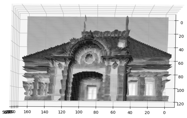
This is a top view, but on viewing sideways we can see the variation in the intensities that make up the image:

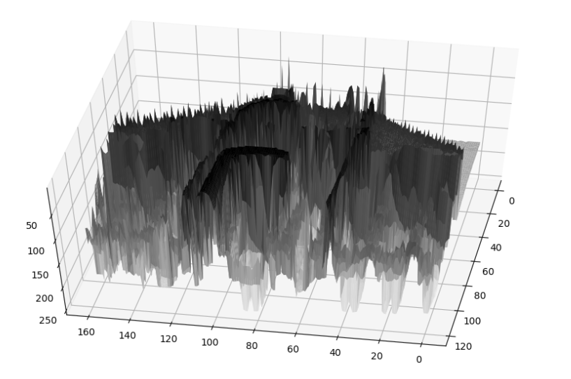
We can see that there are several peaks and image intensities that are not smooth. Let's apply smoothing algorithm, the details for which can be seen in Chapter 3, Image Filtering and Transformations in OpenCV:

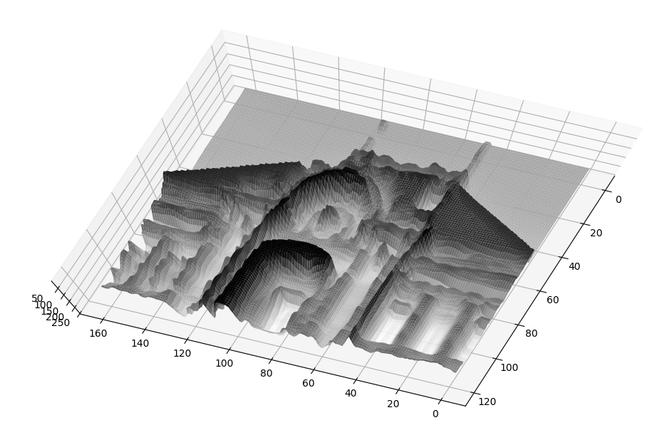
As we can see, pixel intensities form more continuous formations, even though there is no significant change in the object representation. The code to visualize this is as follows (the libraries required to visualize images are described in detail in the Chapter 2, Libraries, Development Platforms, and Datasets, separately):

import numpy as np
import matplotlib.pyplot as plt
from mpl_toolkits.mplot3d import Axes3D
import cv2


# loads and read an image from path to file
img = cv2.imread('../figures/building_sm.png')

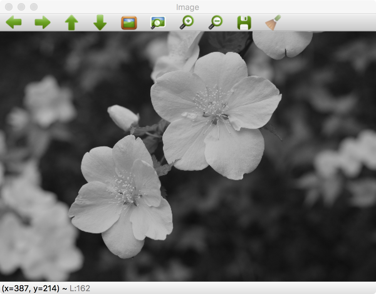
# convert the color to grayscale 
gray = cv2.cvtColor(img, cv2.COLOR_BGR2GRAY)
# resize the image(optional)
gray = cv2.resize(gray, (160, 120))

# apply smoothing operation
gray = cv2.blur(gray,(3,3))

# create grid to plot using numpy
xx, yy = np.mgrid[0:gray.shape[0], 0:gray.shape[1]]

# create the figure
fig = plt.figure()
ax = fig.gca(projection='3d')
ax.plot_surface(xx, yy, gray ,rstride=1, cstride=1, cmap=plt.cm.gray,
        linewidth=1)
# show it
plt.show()

This code uses the following libraries: NumPy, OpenCV, and matplotlib.

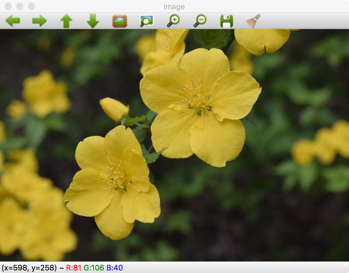
In the further sections of this chapter we will see operations on images using their color properties. Please download the relevant images from the website to view them clearly.

An image, stored in digital format, consists of grid structure with each cell containing a value to represent image. In further sections, we will see different formats for images. For each format, the values represented in the grid cells will have different range of values.

To manipulate an image or use it for further processing, we need to load the image and use it as grid like structure. This is referred to as image input-output operations and we can use OpenCV library to read an image, as follows. Here, change the path to the image file according to use:

import cv2 

# loads and read an image from path to file
img = cv2.imread('../figures/flower.png')

# displays previous image 
cv2.imshow("Image",img)

# keeps the window open until a key is pressed
cv2.waitKey(0)

# clears all window buffers
cv2.destroyAllWindows()

The resulting image is shown in the following screenshot:

Here, we read the image in BGR color format where B is blue, G is green, and R is red. Each pixel in the output is collectively represented using the values of each of the colors. An example of the pixel location and its color values is shown in the previous figure bottom.

An image is made up pixels and is usually visualized according to the value stored. There is also an additional property that makes different kinds of image. Each of the value stored in a pixel is linked to a fixed representation. For example, a pixel value of ten can represent gray intensity value ten or blue color intensity value 10 and so on. It is therefore important to understand different color types and their conversion. In this section, we will see color types and conversions using OpenCV:

• Grayscale: This is a simple one channel image with values ranging from 0 to 255 that represent the intensity of pixels. The previous image can be converted to grayscale, as follows:

import cv2 

# loads and read an image from path to file
img = cv2.imread('../figures/flower.png')

# convert the color to grayscale 
gray = cv2.cvtColor(img, cv2.COLOR_BGR2GRAY)

# displays previous image 
cv2.imshow("Image",gray)

# keeps the window open until a key is pressed
cv2.waitKey(0)

# clears all window buffers
cv2.destroyAllWindows()

The resulting image is as shown in the following screenshot:

• HSV and HLS: These are another representation of color representing H is hue, S is saturation, V is value, and L is lightness. These are motivated by the human perception system. An example of image conversion for these is as follows:

# convert the color to hsv 
hsv = cv2.cvtColor(img, cv2.COLOR_BGR2HSV)

# convert the color to hls 
hls = cv2.cvtColor(img, cv2.COLOR_BGR2HLS)

This conversion is as shown in the following figure, where an input image read in BGR format is converted to each of the HLS (on left) and HSV (on right) color types:

• LAB color space: Denoted L for lightness, A for green-red colors, and B for blue-yellow colors, this consists of all perceivable colors. This is used to convert between one type of color space (for example, RGB) to others (such as CMYK) because of its device independence properties. On devices where the format is different to that of the image that is sent, the incoming image color space is first converted to LAB and then to the corresponding space available on the device. The output of converting an RGB image is as follows: