

NumPy is the fundamental package supported for presenting and computing data with high performance in Python. It provides some interesting features as follows:
- Extension package to Python for multidimensional arrays (
ndarrays), various derived objects (such as masked arrays), matrices providing vectorization operations, and broadcasting capabilities. Vectorization can significantly increase the performance of array computations by taking advantage of Single Instruction Multiple Data (SIMD) instruction sets in modern CPUs. - Fast and convenient operations on arrays of data, including mathematical manipulation, basic statistical operations, sorting, selecting, linear algebra, random number generation, discrete Fourier transforms, and so on.
- Efficiency tools that are closer to hardware because of integrating C/C++/Fortran code.
An array can be used to contain values of a data object in an experiment or simulation step, pixels of an image, or a signal recorded by a measurement device. For example, the latitude of the Eiffel Tower, Paris is 48.858598 and the longitude is 2.294495. It can be presented in a NumPy array object as p:
This is a manual construction of an array using the np.array function. The standard convention to import NumPy is as follows:
You can, of course, put from numpy import * in your code to avoid having to write np. However, you should be careful with this habit because of the potential code conflicts (further information on code conventions can be found in the Python Style Guide, also known as PEP8, at https://www.python.org/dev/peps/pep-0008/).
There are two requirements of a NumPy array: a fixed size at creation and a uniform, fixed data type, with a fixed size in memory. The following functions help you to get information on the p matrix:
>>> p.ndim    # getting dimension of array p
1
>>> p.shape   # getting size of each array dimension
(2,)
>>> len(p)    # getting dimension length of array p
2
>>> p.dtype    # getting data type of array p
dtype('float64')
There are five basic numerical types including Booleans (bool), integers (int), unsigned integers (uint), floating point (float), and complex. They indicate how many bits are needed to represent elements of an array in memory. Besides that, NumPy also has some types, such as intc and intp, that have different bit sizes depending on the platform.
See the following table for a listing of NumPy's supported data types:
|
Type |
Type code |
Description |
Range of value |
|---|---|---|---|
|
|
Boolean stored as a byte |
True/False | |
|
|
Similar to C int (int32 or int 64) | ||
|
|
Integer used for indexing (same as C size_t) | ||
|
|
i1, u1 |
Signed and unsigned 8-bit integer types |
int8: (-128 to 127) uint8: (0 to 255) |
|
|
i2, u2 |
Signed and unsigned 16-bit integer types |
int16: (-32768 to 32767) uint16: (0 to 65535) |
|
|
I4, u4 |
Signed and unsigned 32-bit integer types |
int32: (-2147483648 to 2147483647 uint32: (0 to 4294967295) |
|
|
i8, u8 |
Signed and unsigned 64-bit integer types |
Int64: (-9223372036854775808 to 9223372036854775807) uint64: (0 to 18446744073709551615) |
|
|
f2 |
Half precision float: sign bit, 5 bits exponent, and 10b bits mantissa | |
|
|
f4 / f |
Single precision float: sign bit, 8 bits exponent, and 23 bits mantissa | |
|
|
f8 / d |
Double precision float: sign bit, 11 bits exponent, and 52 bits mantissa | |
|
|
c8, c16, c32 |
Complex numbers represented by two 32-bit, 64-bit, and 128-bit floats | |
|
|
0 |
Python object type | |
|
|
S |
Fixed-length string type |
Declare a string |
|
|
U |
Fixed-length Unicode type |
Similar to string_ example, we have 'U10' |
We can easily convert or cast an array from one dtype to another using the astype method:
There are various functions provided to create an array object. They are very useful for us to create and store data in a multidimensional array in different situations.
|
Function |
Description |
Example |
|---|---|---|
|
|
Create a new array of the given shape and type, without initializing elements |
>>> np.empty([3,2], dtype=np.float64)
array([[0., 0.], [0., 0.], [0., 0.]])
>>> a = np.array([[1, 2], [4, 3]])
>>> np.empty_like(a)
array([[0, 0], [0, 0]])
|
|
|
Create a NxN identity matrix with ones on the diagonal and zero elsewhere |
>>> np.eye(2, dtype=np.int)
array([[1, 0], [0, 1]])
|
|
|
Create a new array with the given shape and type, filled with 1s for all elements |
>>> np.ones(5)
array([1., 1., 1., 1., 1.])
>>> np.ones(4, dtype=np.int)
array([1, 1, 1, 1])
>>> x = np.array([[0,1,2], [3,4,5]])
>>> np.ones_like(x)
array([[1, 1, 1],[1, 1, 1]])
|
|
|
This is similar to |
>>> np.zeros(5)
array([0., 0., 0., 0-, 0.])
>>> np.zeros(4, dtype=np.int)
array([0, 0, 0, 0])
>>> x = np.array([[0, 1, 2], [3, 4, 5]])
>>> np.zeros_like(x)
array([[0, 0, 0],[0, 0, 0]])
|
|
|
Create an array with even spaced values in a given interval |
>>> np.arange(2, 5)
array([2, 3, 4])
>>> np.arange(4, 12, 5)
array([4, 9])
|
|
|
Create a new array with the given shape and type, filled with a selected value |
>>> np.full((2,2), 3, dtype=np.int)
array([[3, 3], [3, 3]])
>>> x = np.ones(3)
>>> np.full_like(x, 2)
array([2., 2., 2.])
|
|
|
Create an array from the existing data |
>>> np.array([[1.1, 2.2, 3.3], [4.4, 5.5, 6.6]])
array([1.1, 2.2, 3.3], [4.4, 5.5, 6.6]])
|
|
|
Convert the input to an array |
>>> a = [3.14, 2.46]
>>> np.asarray(a)
array([3.14, 2.46])
|
|
|
Return an array copy of the given object |
>>> a = np.array([[1, 2], [3, 4]])
>>> np.copy(a)
array([[1, 2], [3, 4]])
|
|
|
Create 1-D array from a string or text |
>>> np.fromstring('3.14 2.17', dtype=np.float, sep=' ')
array([3.14, 2.17])
|
As with other Python sequence types, such as lists, it is very easy to access and assign a value of each array's element:
As another example, if our array is multidimensional, we need tuples of integers to index an item:
We call b and c as array slices, which are views on the original one. It means that the data is not copied to b or c, and whenever we modify their values, it will be reflected in the array a as well:
Besides indexing with slices, NumPy also supports indexing with Boolean or integer arrays (masks). This method is called fancy indexing. It creates copies, not views.
First, we take a look at an example of indexing with a Boolean mask array:
The second example is an illustration of using integer masks on arrays:
Tip
You can download the example code files for all Packt books you have purchased from your account at http://www.packtpub.com. If you purchased this book elsewhere, you can visit http://www.packtpub.com/support and register to have the files e-mailed directly to you.
We are getting familiar with creating and accessing ndarrays. Now, we continue to the next step, applying some mathematical operations to array data without writing any for loops, of course, with higher performance.
Scalar operations will propagate the value to each element of the array:
All arithmetic operations between arrays apply the operation element wise:
Also, here are some examples of comparisons and logical operations:
Many helpful array functions are supported in NumPy for analyzing data. We will list some part of them that are common in use. Firstly, the transposing function is another kind of reshaping form that returns a view on the original data array without copying anything:
See the following table for a listing of array functions:
|
Function |
Description |
Example |
|---|---|---|
|
|
Trigonometric and hyperbolic functions |
>>> a = np.array([0.,30., 45.])
>>> np.sin(a * np.pi / 180)
array([0., 0.5, 0.7071678])
|
|
|
Rounding elements of an array to the given or nearest number |
>>> a = np.array([0.34, 1.65])
>>> np.round(a)
array([0., 2.])
|
|
|
Computing the exponents and logarithms of an array |
>>> np.exp(np.array([2.25, 3.16]))
array([9.4877, 23.5705])
|
|
|
Set of arithmetic functions on arrays |
>>> a = np.arange(6)
>>> x1 = a.reshape(2,3)
>>> x2 = np.arange(3)
>>> np.multiply(x1, x2)
array([[0,1,4],[0,4,10]])
|
|
|
Perform elementwise comparison: >, >=, <, <=, ==, != |
>>> np.greater(x1, x2)
array([[False, False, False], [True, True, True]], dtype = bool)
|
With the NumPy package, we can easily solve many kinds of data processing tasks without writing complex loops. It is very helpful for us to control our code as well as the performance of the program. In this part, we want to introduce some mathematical and statistical functions.
See the following table for a listing of mathematical and statistical functions:
|
Function |
Description |
Example |
|---|---|---|
|
|
Calculate the sum of all the elements in an array or along the axis |
>>> a = np.array([[2,4], [3,5]])
>>> np.sum(a, axis=0)
array([5, 9])
|
|
|
Compute the product of array elements over the given axis |
>>> np.prod(a, axis=1)
array([8, 15])
|
|
|
Calculate the discrete difference along the given axis |
>>> np.diff(a, axis=0)
array([[1,1]])
|
|
|
Return the gradient of an array |
>>> np.gradient(a)
[array([[1., 1.], [1., 1.]]), array([[2., 2.], [2., 2.]])]
|
|
|
Return the cross product of two arrays |
>>> b = np.array([[1,2], [3,4]])
>>> np.cross(a,b)
array([0, -3])
|
|
|
Return standard deviation and variance of arrays |
>>> np.std(a)
1.1180339
>>> np.var(a)
1.25
|
|
|
Calculate arithmetic mean of an array |
>>> np.mean(a)
3.5
|
|
|
Return elements, either from x or y, that satisfy a condition |
>>> np.where([[True, True], [False, True]], [[1,2],[3,4]], [[5,6],[7,8]])
array([[1,2], [7, 4]])
|
|
|
Return the sorted unique values in an array |
>>> id = np.array(['a', 'b', 'c', 'c', 'd'])
>>> np.unique(id)
array(['a', 'b', 'c', 'd'], dtype='|S1')
|
|
|
Compute the sorted and common elements in two arrays |
>>> a = np.array(['a', 'b', 'a', 'c', 'd', 'c'])
>>> b = np.array(['a', 'xyz', 'klm', 'd'])
>>> np.intersect1d(a,b)
array(['a', 'd'], dtype='|S3')
|
Arrays are saved by default in an uncompressed raw binary format, with the file extension .npy by the np.save function:
Arrays are saved by default in an uncompressed raw binary format, with the file extension .npy by the np.save function:
Linear algebra is a branch of mathematics concerned with vector spaces and the mappings between those spaces. NumPy has a package called linalg that supports powerful linear algebra functions. We can use these functions to find eigenvalues and eigenvectors or to perform singular value decomposition:
The following table will summarise some commonly used functions in the numpy.linalg package:
|
Function |
Description |
Example |
|---|---|---|
|
|
Calculate the dot product of two arrays |
>>> a = np.array([[1, 0],[0, 1]])
>>> b = np.array( [[4, 1],[2, 2]])
>>> np.dot(a,b)
array([[4, 1],[2, 2]])
|
|
|
Calculate the inner and outer product of two arrays |
>>> a = np.array([1, 1, 1])
>>> b = np.array([3, 5, 1])
>>> np.inner(a,b)
9
|
|
|
Find a matrix or vector norm |
>>> a = np.arange(3)
>>> np.linalg.norm(a)
2.23606
|
|
|
Compute the determinant of an array |
>>> a = np.array([[1,2],[3,4]])
>>> np.linalg.det(a)
-2.0
|
|
|
Compute the inverse of a matrix |
>>> a = np.array([[1,2],[3,4]])
>>> np.linalg.inv(a)
array([[-2., 1.],[1.5, -0.5]])
|
|
|
Calculate the QR decomposition |
>>> a = np.array([[1,2],[3,4]])
>>> np.linalg.qr(a)
(array([[0.316, 0.948], [0.948, 0.316]]), array([[ 3.162, 4.427], [ 0., 0.632]]))
|
|
|
Compute the condition number of a matrix |
>>> a = np.array([[1,3],[2,4]])
>>> np.linalg.cond(a)
14.933034
|
|
|
Compute the sum of the diagonal element |
>>> np.trace(np.arange(6)).
reshape(2,3))
4
|
An important part of any simulation is the ability to generate random numbers. For this purpose, NumPy provides various routines in the submodule random. It uses a particular algorithm, called the Mersenne Twister, to generate pseudorandom numbers.
An array of random numbers in the [0.0, 1.0] interval can be generated as follows:
NumPy also provides for many other distributions, including the Beta, bionomial, chi-square, Dirichlet, exponential, F, Gamma, geometric, or Gumbel.
|
Function |
Description |
Example |
|---|---|---|
|
|
Draw samples from a binomial distribution (n: number of trials, p: probability) |
>>> n, p = 100, 0.2
>>> np.random.binomial(n, p, 3)
array([17, 14, 23])
|
|
|
Draw samples using a Dirichlet distribution |
>>> np.random.dirichlet(alpha=(2,3), size=3)
array([[0.519, 0.480], [0.639, 0.36],
 [0.838, 0.161]])
|
|
|
Draw samples from a Poisson distribution |
>>> np.random.poisson(lam=2, size= 2)
array([4,1])
|
|
|
Draw samples using a normal Gaussian distribution |
>>> np.random.normal
(loc=2.5, scale=0.3, size=3)
array([2.4436, 2.849, 2.741)
|
|
|
Draw samples using a uniform distribution |
>>> np.random.uniform(
low=0.5, high=2.5, size=3)
array([1.38, 1.04, 2.19[)
|
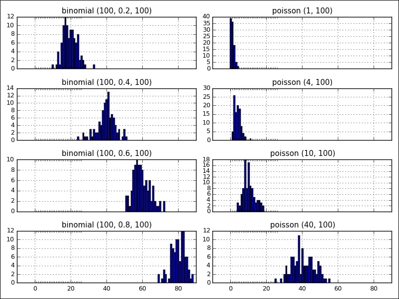
The following figure shows two distributions, binomial and poisson , side by side with various parameters (the visualization was created with matplotlib, which will be covered in Chapter 4, Data Visualization):
Then, we are getting familiar with some common functions and operations on ndarray.
Exercise 2: What is the difference between np.dot(a, b) and (a*b)?