Using computational graphs
Through evolution, humans have found that graphing the neural network gives us the power of reducing complexity to the bare minimum. A computational graph describes the data flow in the network through operations.
A graph, which is made by a group of nodes and edges connecting them, is a decades-old data structure that is still heavily used in several different implementations and is a data structure that will be valid probably until humans cease to exist. In computational graphs, nodes represent the tensors and edges represent the relationship between them.
Computational graphs help us to solve the mathematics and make the big networks intuitive. Neural networks, no matter how complex or big they are, are a group of mathematical operations. The obvious approach to solving an equation is to divide the equation into smaller units and pass the output of one to another and so on. The idea behind the graph approach is the same. You consider the operations inside the network as nodes and map them to a graph with relations between nodes representing the transition from one operation to another.
Computational graphs are at the core of all current advances in artificial intelligence. They made the foundation of deep learning frameworks. All the deep learning frameworks existing now do computations using the graph approach. This helps the frameworks to find the independent nodes and do their computation as a separate thread or process. Computational graphs help with doing the backpropagation as easily as moving from the child node to previous nodes, and carrying the gradients along while traversing back. This operation is called automatic differentiation, which is a 40-year-old idea. Automatic differentiation is considered one of the 10 great numerical algorithms in the last century. Specifically, reverse-mode automatic differentiation is the core idea used behind computational graphs for doing backpropagation. PyTorch is built based on reverse-mode auto differentiation, so all the nodes keep the operation information with them until the control reaches the leaf node. Then the backpropagation starts from the leaf node and traverses backward. While moving back, the flow takes the gradient along with it and finds the partial derivatives corresponding to each node. In 1970, Seppo Linnainmaa, a Finnish mathematician and computer scientist, found that automatic differentiation can be used for algorithm verification. A lot of the other parallel efforts were recorded on the same concepts almost at the same time.
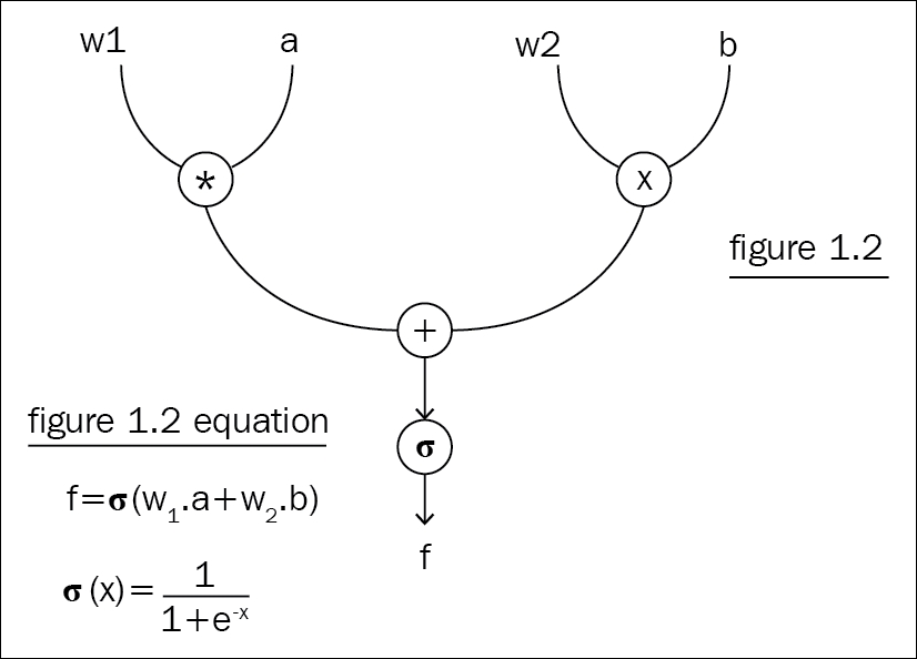
In deep learning, neural networks are for solving a mathematical equation. Regardless of how complex the task is, everything comes down to a giant mathematical equation, which you'll solve by optimizing the parameters of the neural network. The obvious way to solve it is "by hand." Consider solving the mathematical equation for ResNet with around 150 layers of a neural network; it is sort of impossible for a human being to iterate over such graphs thousands of times, doing the same operations manually each time to optimize the parameters. Computational graphs solve this problem by mapping all operations to a graph, level by level, and solving each node at a time. Figure 1.2 shows a simple computational graph with three operators.
The matrix multiplication operator on both sides gives two matrices as output, and they go through an addition operator, which in turn goes through another sigmoid operator. The whole graph is, in fact, trying to solve this equation:
However, the moment you map it to a graph, everything becomes crystal clear. You can visualize and understand what is happening and easily code it up because the flow is right in front of you.
All deep learning frameworks are built on the foundation of automatic differentiation and computational graphs, but there are two inherently different approaches for the implementation–static and dynamic graphs.
The traditional way of approaching neural network architecture is with static graphs. Before doing anything with the data you give, the program builds the forward and backward pass of the graph. Different development groups have tried different approaches. Some build the forward pass first and then use the same graph instance for the forward and backward pass. Another approach is to build the forward static graph first, and then create and append the backward graph to the end of the forward graph, so that the whole forward-backward pass can be executed as a single graph execution by taking the nodes in chronological order.
Static graphs come with certain inherent advantages over other approaches. Since you are restricting the program from dynamic changes, your program can make assumptions related to memory optimization and parallel execution while executing the graph. Memory optimization is the key aspect that framework developers worry about through most of their development time, and the reason is the humungous scope of optimizing memory and the subtleties that come along with those optimizations. Apache MXNet developers have written an amazing blog [3] talking about this in detail.
The neural network for predicting the XOR output in TensorFlow's static graph API is given as follows. This is a typical example of how static graphs execute. Initially, we declare all the input placeholders and then build the graph. If you look carefully, nowhere in the graph definition are we passing the data into it. Input variables are actually placeholders expecting data sometime in the future. Though the graph definition looks like we are doing mathematical operations on the data, we are actually defining the process, and that's when TensorFlow builds the optimized graph implementation using the internal engine:
Once the interpreter finishes reading the graph definition, we start looping it through the data:
We start a TensorFlow session next. That's the only way you can interact with the graph you built beforehand. Inside the session, you loop through your data and pass the data to your graph using the session.run method. So, your input should be of the same size as you defined in the graph.
If you have forgotten what XOR is, the following table should give you enough information to recollect it from memory:
The imperative style of programming has always had a larger user base, as the program flow is intuitive to any developer. Dynamic capability is a good side effect of imperative-style graph building. Unlike static graphs, dynamic graph architecture doesn't build the graph before the data pass. The program will wait for the data to come and build the graph as it iterates through the data. As a result, each iteration through the data builds a new graph instance and destroys it once the backward pass is done. Since the graph is being built for each iteration, it doesn't depend on the data size or length or structure. Natural language processing is one of the fields that needs this kind of approach.
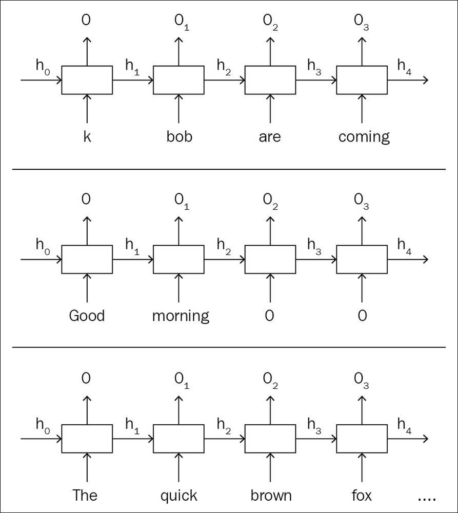
For example, if you are trying to do sentiment analysis on thousands of sentences, with a static graph you need to hack and make workarounds. In a vanilla recurrent neural network (RNN) model, each word goes through one RNN unit, which generates output and the hidden state. This hidden state will be given to the next RNN, which processes the next word in the sentence. Since you made a fixed length slot while building your static graph, you need to augment your short sentences and cut down long sentences.
The static graph given in the example shows how the data needs to be formatted for each iteration such that it won't break the prebuilt graph. However, in the dynamic graph, the network is flexible such that it gets created each time you pass the data, as shown in the preceding diagram.
The dynamic capability comes with a cost. Your graph cannot be preoptimized based on assumptions and you have to pay for the overhead of graph creation at each iteration. However, PyTorch is built to reduce the cost as much as possible. Since preoptimization is not something that a dynamic graph is capable of doing, PyTorch developers managed to bring down the cost of instant graph creation to a negligible amount. With all the optimization going into the core of PyTorch, it has proved to be faster than several other frameworks for specific use cases, even while offering the dynamic capability.
Following is a code snippet written in PyTorch for the same XOR operation we developed earlier in TensorFlow:
In the PyTorch code, the input variable definition is not creating placeholders; instead, it is wrapping the variable object onto your input. The graph definition is not executing once; instead, it is inside your loop and the graph is being built for each iteration. The only information you share between each graph instance is your weight matrix, which is what you want to optimize.
In this approach, if your data size or shape is changing while you're looping through it, it's absolutely fine to run that new-shaped data through your graph because the newly created graph can accept the new shape. The possibilities do not end there. If you want to change the graph's behavior dynamically, you can do that too. The example given in the recursive neural network session in Chapter 5, Sequential Data Processing, is built on this idea.


 Free Chapter