

The next descriptive statistics covered will be the mean, also called the average, and standard deviation. In this section, we will use the sum and length functions to compose the mean of a dataset. We'll also explore the sum and length functions; compose our mean function; and then use that mean function in order to compose a standard deviation function. Finally, we're going to compute the mean and standard deviation of the 2015 away-team runs using our function.
The mean is a summary statistic that gives you a rough idea of the middle values of the dataset, while not truly being the middle of a dataset:

The mean is trivial to calculate and thus it is frequently used, and it is the sum of that dataset divided by the number of values in that dataset.
We will also discuss sample standard deviation, which is the mean distance from the mean and a measure of a dataset spread. The approach that we will be using is known as the sample standard deviation. I have presented the function here for your reference:

Now, let's go over to our Linux environment. We left off last section discussing the range of a dataset. Let's add a new import now, Data.Maybe, as follows:
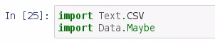
Here, we have added a library. Each time we add libraries, we will restart and rerun all, and it's okay to do this. It will take a moment, and will reload all of our variables.
In order to compute the mean of a dataset, we add up all the values and divide this value by the length of those values. So, in order to find the sum of all the values in a list, we use sum on the awayRuns variable, and we also need to find the length of the awayRuns variable:
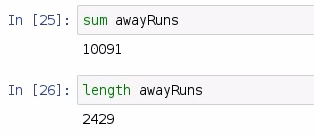
There were 10,091 runs scored in the 2015 season by the away team, and 2,429 games played in that season. We divide the first number by the second, and we get our average; but we need to explore the type of the sum and the length functions:
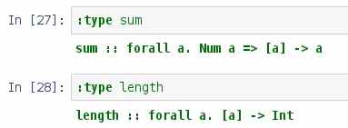
We can see that the sum takes a list of values and returns a value, and the sum inputs and the outputs are bound by the Num type, whereas the inputs on length aren't bound by anything, and they always return an int. The division operator in Haskell doesn't work with int, so what we need to do is to convert the values returned by sum and length to something that we can work with:
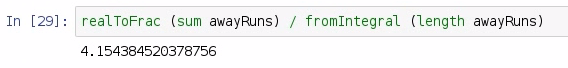
So the function we have used for this is realToFrac, where we pass sum of the away runs divided by fromIntegral, which takes the length of the away runs. So, our average is 4.15 runs per game scored by away teams in the 2015 season. We use this information in order to compose our mean function:
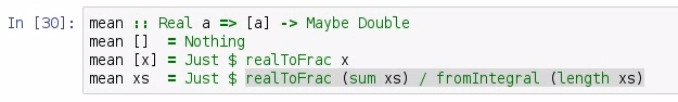
Much like our range function, we have a return type of a double that's been packaged into a Maybe, and we have a list of values that are bound on the Real type. Our function uses pattern matching in order to handle the variety of inputs and outputs that we will likely receive, much like we did with the range function in the last section. So, if we have a list of no values, we return Nothing. Now, it's best that we return Nothing, and not 0, because 0 could be interpreted as a mean of a dataset. If we have a single value, then we're just going to return that value bundled in Just, and if we have a list, then we're actually going to implement the sum and length functions that we described earlier. So, let's test this out:
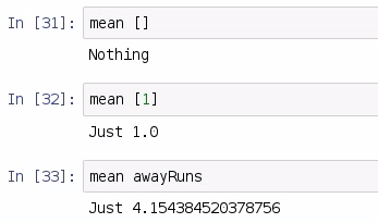
As we can see, if we get the mean of an empty list, we should get Nothing; if we get mean of a single value, we should get that value converted to a double; and if we have mean of a true list, we should get our average, which in our case is 4.15.
Now, any function that uses our mean function is going to have to interpret the value inside of Maybe, so in order to do that, we use a function called fromJust. Now, let's write the code for the standard deviation, as follows:
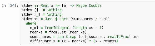
Much like the mean function we wrote earlier, we have our inputs bound by a Real type; and we will be returning a Double packaged to the Maybe. And for historical reasons, we will call this function stdev. Statistical spreadsheet software and statistical packages will call this particular function stdev, which is a recreation of the formula that we saw at the beginning of this section, which produces the sample standard deviation. It's important to note that the sample standard deviation requires at least two values in order to compute a spread. You can't very well compute a spread with one value, and so we need to use pattern matching in order to detect that, thus if we have an empty list, we return Nothing. If we have a list of just one item, we still return Nothing. After that, we have actually implemented the formula necessary for the sample standard deviation. Let's do a few tests:
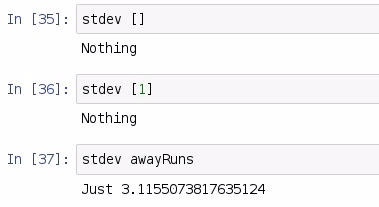
So, the standard deviation of a blank list is Nothing; the standard deviation of a single item is still Nothing; and the standard deviation of our awayRuns is 3.12. With this information, we are going to take our average which is 4.15, and we will subtract it with 3.12 and we will also add 3.12 to it:
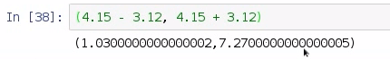
We can say that one standard deviation range of our away-team runs for the 2015 season is 1.03 runs to 7.27 runs; and that gives us a good idea of where the majority of the scores were for away teams in the 2015 season. So, in this section, we looked at the mean and the standard deviations of a dataset. We implemented the functions; we discussed the sum and the length functions necessary for those functions; and then we did a few examples of how we could find the mean and standard deviation with the functions that we had prototyped. In the next section, we will be discussing the median of a dataset.