Support Vector Regression

SVMs are binary classifiers and are usually used in classification problems (you will learn more about this in Chapter 3, An Introduction to Classification). An SVM classifier takes data and tries to predict which class it belongs to. Once the classification of a data point is determined, it gets labeled. But SVMs can also be used for regression; that is, instead of labeling data, it can predict future values in a series.

The SVR model uses the space between our data as a margin of error. Based on the margin of error, it makes predictions regarding future values.

If the margin of error is too small, we risk overfitting the existing dataset. If the margin of error is too big, we risk underfitting the existing dataset.

In the case of a classifier, the kernel describes the surface dividing the state space, whereas, in a regression, the kernel measures the margin of error. This kernel can use a linear model, a polynomial model, or many other possible models. The default kernel is RBF, which stands for Radial Basis Function.

SVR is an advanced topic that is outside the scope of this book. Therefore, we will only stick to an easy walk-through as an opportunity to try out another regression model on our data.

We can reuse the code from Exercise 2.03, Preparing the Quandl Data for Prediction, up to Step 11:

import quandl
import numpy as np
from sklearn import preprocessing
from sklearn import model_selection
from sklearn import linear_model
from matplotlib import pyplot as plot
 
data_frame = quandl.get(“YALE/SPCOMP”, \
                        start_date=”1950-01-01”, \
                        end_date=”2019-12-31”)
data_frame = data_frame[['Long Interest Rate', \
                         'Real Price', 'Real Dividend']]
data_frame.fillna(method='ffill', inplace=True)
data_frame['Real Price Label'] = data_frame['Real Price'].shift(-3)
features = np.array(data_frame.drop('Real Price Label', 1))
scaled_features = preprocessing.scale(features)
scaled_features_latest_3 = scaled_features[-3:]
scaled_features = scaled_features[:-3]
data_frame.dropna(inplace=True)
label = np.array(data_frame['Real Price Label'])
(features_train, features_test, label_train, label_test) = \
model_selection.train_test_split(scaled_features, label, \
                                 test_size=0.1, \
                                 random_state=8)

Then, we can perform a regression with svm by simply changing the linear model to a support vector model by using the svm method from sklearn:

from sklearn import svm
model = svm.SVR()
model.fit(features_train, label_train)

As you can see, performing an SVR is exactly the same as performing a linear regression, with the exception of defining the model as svm.SVR().

Finally, we can predict and measure the performance of our model:

label_predicted = model.predict(features_test)
model.score(features_test, label_test)

The output is as follows:

0.03262153550014424

As you can see, the score or R2 is quite low, our SVR's parameters need to be optimized in order to increase the accuracy of the model.

Support Vector Machines with a 3-Degree Polynomial Kernel

Let's switch the kernel of the SVM to a polynomial function (the default degree is 3) and measure the performance of the new model:

model = svm.SVR(kernel='poly') 
model.fit(features_train, label_train) 
label_predicted = model.predict(features_test) 
model.score(features_test, label_test)

The output is as follows:

0.44465054598560627

We managed to increase the performance of the SVM by simply changing the kernel function to a polynomial function; however, the model still needs a lot of tuning to reach the same performance as the linear regression models.

Activity 2.01: Boston House Price Prediction with Polynomial Regression of Degrees 1, 2, and 3 on Multiple Variables

In this activity, you will need to perform linear polynomial regression of degrees 1, 2, and 3 with scikit-learn and find the best model. You will work on the Boston House Prices dataset. The Boston House Price dataset is very famous and has been used as an example for research on regression models.

Note

More details about the Boston House Prices dataset can be found at https://archive.ics.uci.edu/ml/machine-learning-databases/housing/.

The dataset file can also be found in our GitHub repository: https://packt.live/2V9kRUU.

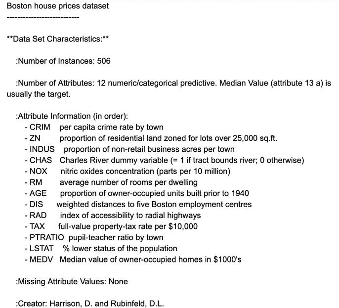
You will need to predict the prices of houses in Boston (label) based on their characteristics (features). Your main goal will be to build 3 linear models using polynomial regressions of degrees 1, 2, and 3 with all the features of the dataset. You can find the following dataset description:

Figure 2.26: Boston housing dataset description

We will define our label as the MEDV field, which is the median value of the house in $1,000s. All of the other fields will be used as our features for our models. As this dataset does not contain any missing values, we won't have to replace missing values as we did in the previous exercises.

The following steps will help you to complete the activity:

1. Open a Jupyter Notebook.
2. Import the required packages and load the Boston House Prices data into a DataFrame.
3. Prepare the dataset for prediction by converting the label and features into NumPy arrays and scaling the features.
4. Create three different sets of features by transforming the scaled features into suitable formats for each of the polynomial regressions.
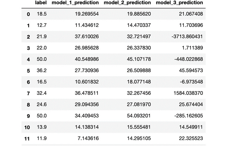
5. Split the data into training and testing sets with random state = 8.
6. Perform a polynomial regression of degree 1 and evaluate whether the model is overfitting.
7. Perform a polynomial regression of degree 2 and evaluate whether the model is overfitting.
8. Perform a polynomial regression of degree 3 and evaluate whether the model is overfitting.
9. Compare the predictions of the three models against the label on the testing set.

The expected output is this:

Figure 2.27: Expected output based on the predictions

Note

The solution for this activity can be found via this link.