-
Book Overview & Buying
-
Table Of Contents

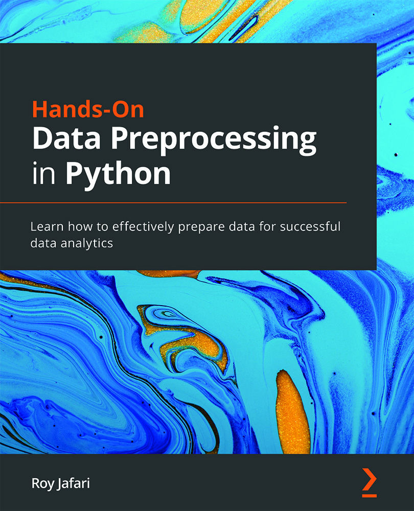
Hands-On Data Preprocessing in Python
By :
Hands-On Data Preprocessing in Python
By:
Overview of this book
Hands-On Data Preprocessing is a primer on the best data cleaning and preprocessing techniques, written by an expert who’s developed college-level courses on data preprocessing and related subjects.
With this book, you’ll be equipped with the optimum data preprocessing techniques from multiple perspectives, ensuring that you get the best possible insights from your data.
You'll learn about different technical and analytical aspects of data preprocessing – data collection, data cleaning, data integration, data reduction, and data transformation – and get to grips with implementing them using the open source Python programming environment.
The hands-on examples and easy-to-follow chapters will help you gain a comprehensive articulation of data preprocessing, its whys and hows, and identify opportunities where data analytics could lead to more effective decision making. As you progress through the chapters, you’ll also understand the role of data management systems and technologies for effective analytics and how to use APIs to pull data.
By the end of this Python data preprocessing book, you'll be able to use Python to read, manipulate, and analyze data; perform data cleaning, integration, reduction, and transformation techniques, and handle outliers or missing values to effectively prepare data for analytic tools.
Table of Contents (24 chapters)
Preface

Part 1:Technical Needs
 Free Chapter
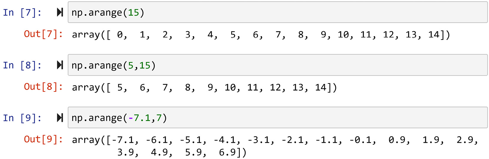
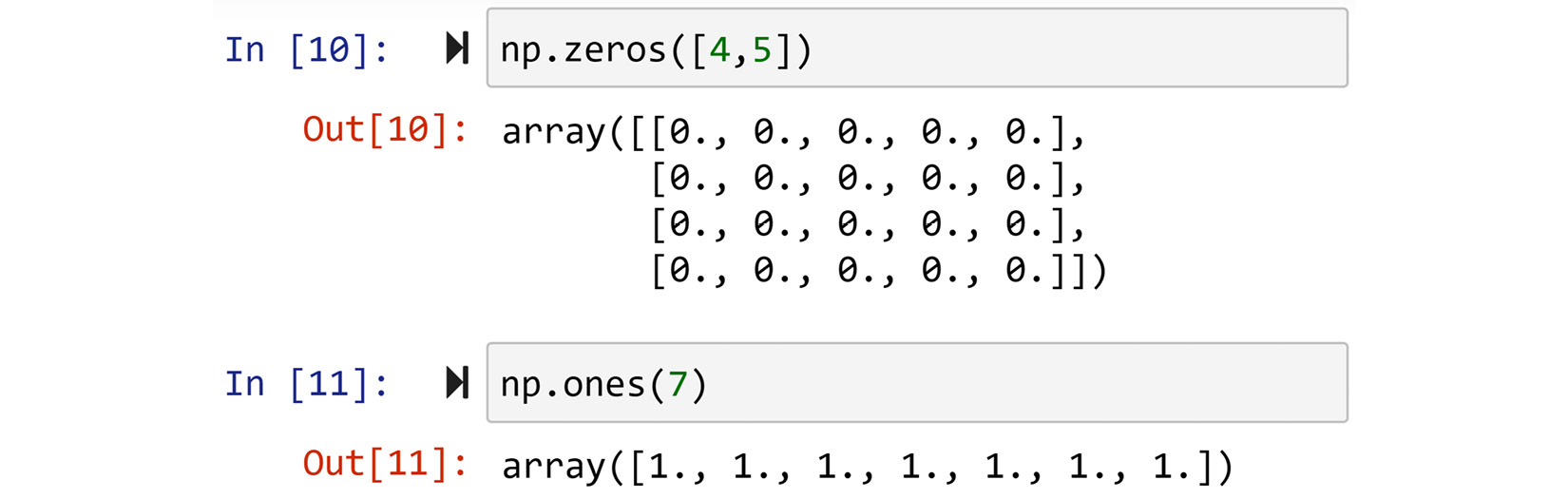
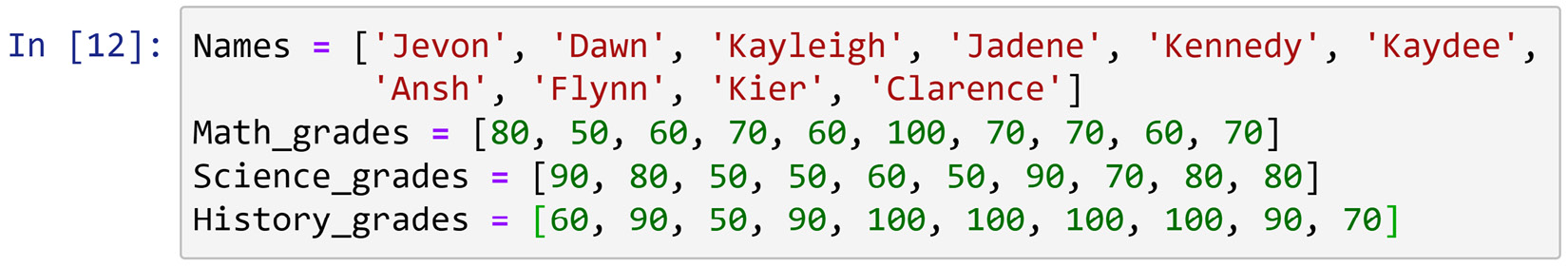
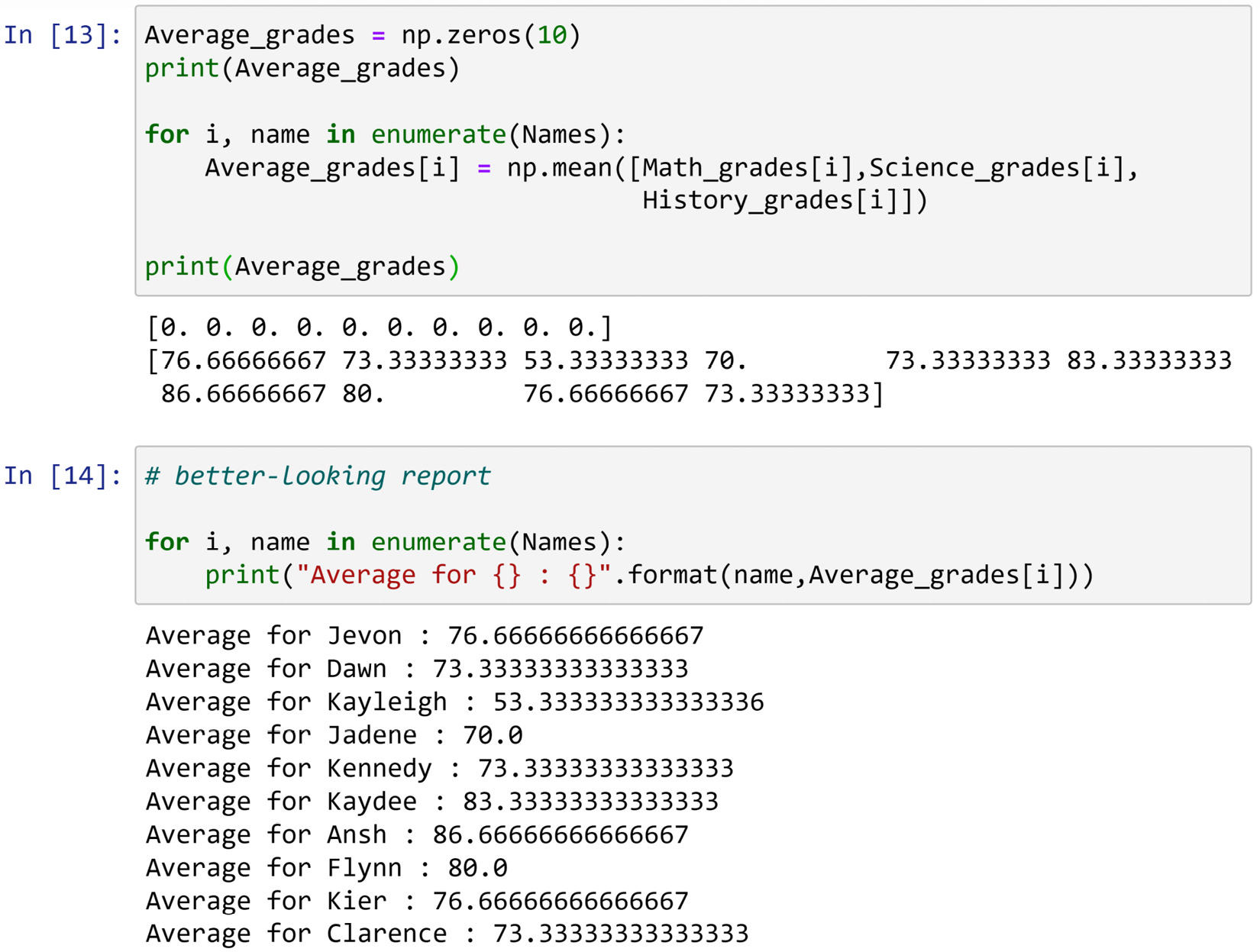
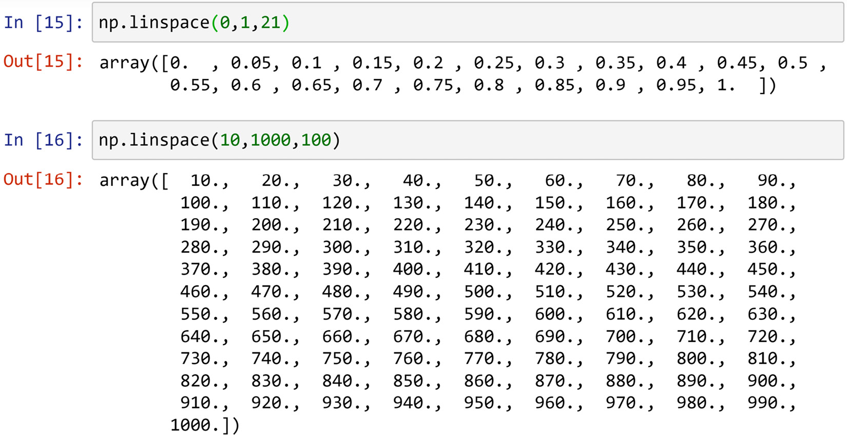
Chapter 1: Review of the Core Modules of NumPy and Pandas
Chapter 2: Review of Another Core Module – Matplotlib
Chapter 3: Data – What Is It Really?
Chapter 4: Databases
Part 2: Analytic Goals
Chapter 5: Data Visualization
Chapter 6: Prediction
Chapter 7: Classification
Chapter 8: Clustering Analysis
Part 3: The Preprocessing
Chapter 9: Data Cleaning Level I – Cleaning Up the Table
Chapter 10: Data Cleaning Level II – Unpacking, Restructuring, and Reformulating the Table
Chapter 11: Data Cleaning Level III – Missing Values, Outliers, and Errors
Chapter 12: Data Fusion and Data Integration
Chapter 13: Data Reduction
Chapter 14: Data Transformation and Massaging
Part 4: Case Studies
Chapter 15: Case Study 1 – Mental Health in Tech
Chapter 16: Case Study 2 – Predicting COVID-19 Hospitalizations
Chapter 17: Case Study 3: United States Counties Clustering Analysis
Chapter 18: Summary, Practice Case Studies, and Conclusions
Other Books You May Enjoy


 .
.