Common uses for NLP

One thing that I like the most about NLP is that you are primarily limited by your imagination and what you can do with it. If you are a creative person, you will be able to come up with many ideas that I have not explained.

I will explain some of the common uses of NLP that I have found. Some of this may not typically appear in NLP books, but as a lifelong programmer, when I think of NLP, I automatically think about any programmatic work with string, with a string being a sequence of characters. ABCDEFG is a string, for instance. A is a character.

Note

Please don’t bother writing the code for now unless you just want to experiment with some of your own data. The code in this chapter is just to show what is possible and what the code may look like. We will go much deeper into actual code throughout this book.

True/False – Presence/Absence

This may not fit strictly into NLP, but it is very often a part of any text operation, and this also happens in ML used in NLP, where one-hot encoding is used. Here, we are looking strictly for the presence or absence of something. For instance, as we saw earlier in the chapter, I wanted to count the number of times that Adam and Eve appeared in the Bible. I could have similarly written some simple code to determine whether Adam and Eve were in the Bible at all or whether they were in the book of Exodus.

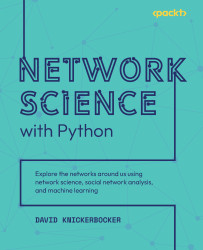
For this example, let’s use this DataFrame that I have set up:

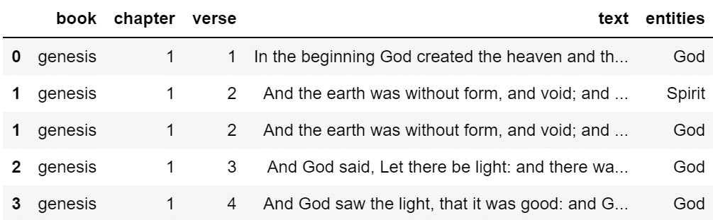
Figure 1.2 – pandas DataFrame containing the entire King James Version text of the Bible

I specifically want to see whether Eve exists as one of the entities in df['entities']. I want to keep the data in a DataFrame, as I have uses for it, so I will just do some pattern matching on the entities field:

check_df['entities'].str.contains('^Eve$')
0        False
1        False
1        False
2        False
3        False
         ...
31101    False
31101    False
31102    False
31102    False
31102    False
Name: entities, Length: 51702, dtype: bool

Here, I am using what is called a regular expression (regex) to look for an exact match on the word Eve. The ^ symbol means that the E in Eve sits at the very beginning of the string, and $ means that the e sits at the very end of the string. This ensures that there is an entity that is exactly named Eve, with nothing before and after. With regex, you have a lot more flexibility than this, but this is a simple example.

In Python, if you have a series of True and False values, .min() will give you False, and .max() will give you True, and that makes sense as another way of looking at True and False is a 1 and 0, and 1 is greater than 0. There are other ways to do this, but I am going to do it this way. So, to see whether Eve is mentioned even once in the whole Bible, I can do the following:

check_df['entities'].str.contains('^Eve$').max()
True

If I want to see if Adam is in the Bible, I can replace Eve with Adam:

check_df['entities'].str.contains('^Adam$').max()
True

Detecting the presence or absence of something in a piece of text can be useful. For instance, if we want to very quickly get a list of Bible verses that are about Eve, we can do the following:

check_df[check_df['entities'].str.contains('^Eve$')]

This will give us a DataFrame of Bible verses mentioning Eve:

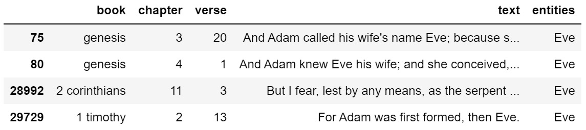
Figure 1.3 – Bible verses containing strict mentions of Eve

If we want to get a list of verses that are about Noah, we can do this:

check_df[check_df['entities'].str.contains('^Noah$')].head(10)

This will give us a DataFrame of Bible verses mentioning Noah:

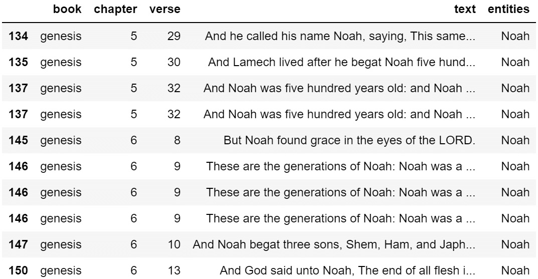
Figure 1.4 – Bible verses containing strict mentions of Noah

I have added .head(10) to only see the first ten rows. With text, I often find myself wanting to see more than the default five rows.

And if we didn’t want to use the entities field, we could look in the text instead.

df[df['text'].str.contains('Eve')]

This will give us a DataFrame of Bible verses where the text of the verse included a mention of Eve.

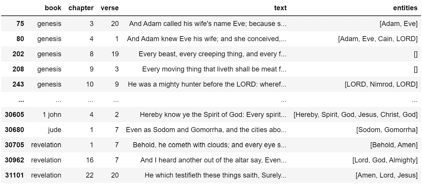
Figure 1.5 – Bible verses containing mentions of Eve

That is where this gets a bit messy. I have already done some of the hard work, extracting entities for this dataset, which I will show how to do in a later chapter. When you are dealing with raw text, regex and pattern matching can be a headache, as shown in the preceding figure. I only wanted the verses that contained Eve, but instead, I got matches for words such as even and every. That’s not what I want.

Anyone who works with text data is going to want to learn the basics of regex. Take heart, though. I have been using regex for over twenty years, and I still very frequently have to Google search to get mine working correctly. I’ll revisit regex, but I hope that you can see that it is pretty simple to determine if a word exists in a string. For something more practical, if you had 400,000 scraped tweets and you were only interested in the ones that were about a specific thing, you could easily use the preceding techniques or regex to look for an exact or close match.

Regular expressions (regex)

I briefly explained regex in the previous section, but there is much more that you can use it for than to simply determine the presence or absence of something. For instance, you can also use regex to extract data from text to enrich your datasets. Let’s look at a data science feed that I scrape:

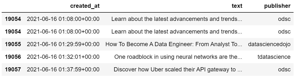
Figure 1.6 – Scraped data science Twitter feed

There’s a lot of value in that text field, but it is difficult to work with in its current form. What if I only want a list of links that are posted every day? What if I want to see the hashtags that are used by the data science community? What if I want to take these tweets and build a social network to analyze who interacts? The first thing we should do is enrich the dataset by extracting things that we want. So, if I wanted to create three new fields that contained lists of hashtags, mentions, and URLs, I could do the following:

df['text'] = df['text'].str.replace('@', ' @')
df['text'] = df['text'].str.replace('#', ' #')
df['text'] = df['text'].str.replace('http', ' http')
df['users'] = df['text'].apply(lambda tweet: [token for token in tweet.split() if token.startswith('@')])
df['tags'] = df['text'].apply(lambda tweet: [token for token in tweet.split() if token.startswith('#')])
df['urls'] = df['text'].apply(lambda tweet: [token for token in tweet.split() if token.startswith('http')])

In the first three lines, I am adding a space behind each mention, hashtag, and URL just to give a little breathing room for splitting. In the next three lines, I am splitting each tweet by space and then applying rules to identify mentions, hashtags, and URLs. In this case, I don’t use fancy logic. Mentions start with @, hashtags start with #, and URLs start with HTTP (to include HTTPS). The result of this code is that I end up with three additional columns, containing lists of users, tags, and URLs.

If I then use explode() on the users, tags, and URLs, I will get a DataFrame where each individual user, tag, and URL has its own row. This is what the DataFrame looks like after explode():

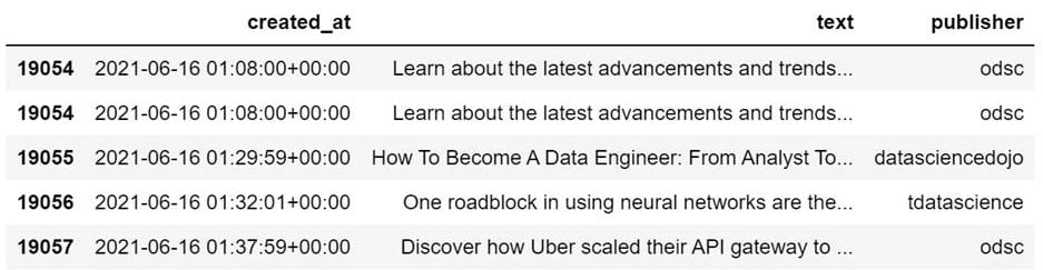
Figure 1.7 – Scraped data science Twitter feed, enriched with users, tags, and URLs

I can then use these new columns to get a list of unique hashtags used:

sorted(df['tags'].dropna().str.lower().unique())
['#',
 '#,',
 '#1',
 '#1.',
 '#10',
 '#10...',
 '#100daysofcode',
 '#100daysofcodechallenge',
 '#100daysofcoding',
 '#15minutecity',
 '#16ways16days',
 '#1bestseller',
 '#1m_ai_talents_in_10_years!',
 '#1m_ai_talents_in_10_yrs!',
 '#1m_ai_talents_in_10yrs',
 '#1maitalentsin10years',
 '#1millionaitalentsin10yrs',
 '#1newrelease',
 '#2'

Clearly, the regex used in my data enrichment is not perfect, as punctuation should not be included in hashtags. That’s something to fix. Be warned, working with human language is very messy and difficult to get perfect. We just have to be persistent to get exactly what we want.

Let’s see what the unique mentions look like. By unique mentions, I mean the deduplicated individual accounts mentioned in tweets:

sorted(df['users'].dropna().str.lower().unique())
['@',
 '@027_7',
 '@0dust_himanshu',
 '@0x72657562656e',
 '@16yashpatel',
 '@18f',
 '@1ethanhansen',
 '@1littlecoder',
 '@1njection',
 '@1wojciechnowak',
 '@20,',
 '@26th_february_2021',
 '@29mukesh89',
 '@2net_software',

That looks a lot better, though @ should not exist alone, the fourth one looks suspicious, and a few of these look like they were mistakenly used as mentions when they should have been used as hashtags. That’s a problem with the tweet text, not the regular expression, most likely, but worth investigating.

I like to lowercase mentions and hashtags so that it is easier to find unique tags. This is often done as preprocessing for NLP.

Finally, let’s get a list of unique URLs mentioned (which can then be used for further scraping):

sorted(df['urls'].dropna().unique())
['http://t.co/DplZsLjTr4',
 'http://t.co/fYzSPkY7Qk',
 'http://t.co/uDclS4EI98',
 'https://t.co/01IIAL6hut',
 'https://t.co/01OwdBe4ym',
 'https://t.co/01wDUOpeaH',
 'https://t.co/026c3qjvcD',
 'https://t.co/02HxdLHPSB',
 'https://t.co/02egVns8MC',
 'https://t.co/02tIoF63HK',
 'https://t.co/030eotd619',
 'https://t.co/033LGtQMfF',
 'https://t.co/034W5ItqdM',
 'https://t.co/037UMOuInk',
 'https://t.co/039nG0jyZr'

This looks very clean. How many URLs was I able to extract?

len(sorted(df['urls'].dropna().unique()))
19790

That’s a lot of links. As this is Twitter data, a lot of URLs are often photos, selfies, YouTube links, and other things that may not be too useful to a researcher, but this is my scraped data science feed, which pulls information from dozens of data science related accounts, so many of these URLs likely include exciting news and research.

Regex allows you to extract additional data from your data and use it to enrich your datasets to do easier or further analysis, and if you extract URLs, you can use that as input for additional scraping.

I’m not going to give a long lesson into regex. There are a whole lot of books dedicated to the topic. It is likely that, eventually, you will need to learn how to use regex. For what we are doing in this book, the preceding regex is probably all you will need, as we are using these tools to build social networks that we can analyze. This book isn’t primarily about NLP. We just use some NLP techniques to create or enrich our data, and then we will use network analysis for everything else.

Word counts

Word counts are also useful, especially when we want to compare things against each other. For instance, we already compared the number of times that Adam and Eve were mentioned in the Bible, but what if we want to see the number of times that all entities are mentioned in the Bible? We can do this the simple way, and we can do this the NLP way. I prefer to do things the simple way, where possible, but frequently, the NLP or graph way ends up being the simpler way, so learn everything that you can and decide for yourself.

We will do this the simple way by counting the number of times entities were mentioned. Let’s use the dataset again and just do some aggregation to see who the most mentioned people are in the Bible. Keep in mind we can do this for any feed that we scrape, so long as we have enriched the dataset to contain a list of mentions. But for this demonstration, I’ll use the Bible.

On the third line, I am keeping entities with a name longer than two characters, effectively dropping some junk entities that ended up in the data. I am using this as a filter:

check_df = df.explode('entities')
check_df.dropna(inplace=True) # dropping nulls
check_df = check_df[check_df['entities'].apply(len) > 2] # dropping some trash that snuck in
check_df['entities'] = check_df['entities'].str.lower()
agg_df = check_df[['entities', 'text']].groupby('entities').count()
agg_df.columns = ['count']
agg_df.sort_values('count', ascending=False, inplace=True)
agg_df.head(10)

This is shown in the following DataFrame:

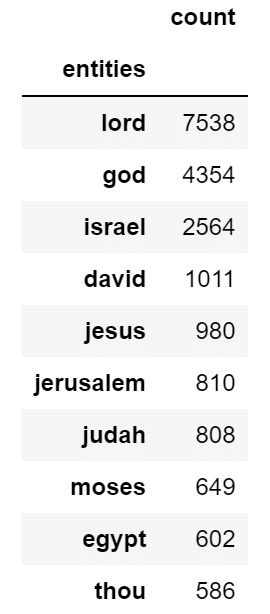
Figure 1.8 – Entity counts across the entire Bible

This looks pretty good. Entities are people, places, and things, and the only oddball in this bunch is the word thou. The reason that snuck in is that in the Bible, often the word thou is capitalized as Thou, which gets tagged as an NNP (Proper Noun) when doing entity recognition and extraction in NLP. However, thou is in reference to You, and so it makes sense. For example, Thou shalt not kill, thou shalt not steal.

If we have the data like this, we can also very easily visualize it for perspective:

agg_df.head(10).plot.barh(figsize=(12, 6), title='Entity Counts by Bible Mentions', legend=False).invert_yaxis()

This will give us a horizontal bar chart of entity counts:

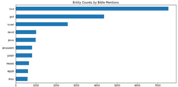
Figure 1.9 – Visualized entity counts across the entire Bible

This is obviously not limited to use on the Bible. If you have any text at all that you are interested in, you can use these techniques to build a deeper understanding. If you want to use these techniques to pursue art, you can. If you want to use these techniques to help fight crime, you can.

Sentiment analysis

This is my favorite technique in all of NLP. I want to know what people are talking about and how they feel about it. This is an often underexplained area of NLP, and if you pay attention to how most people use it, you will see many demonstrations on how to build classifiers that can determine positive or negative sentiment. However, we humans are complicated. We are not just happy or sad. Sometimes, we are neutral. Sometimes we are mostly neutral but more positive than negative. Our feelings are nuanced. One book that I have used a lot for my own education and research into sentiment analysis mentions a study that mapped out human emotions as having primary, secondary, and tertiary emotions (Liu, Sentiment Analysis, 2015, p. 35). Here are a few examples:

Figure 1.10 – A table of primary, secondary, and tertiary emotions

There are a few primary emotions, there are more secondary emotions, and there are many, many more tertiary emotions. Sentiment analysis can be used to try to classify yes/no for any emotion as long as you have training data.

Sentiment analysis doesn’t have to only be used for detecting emotions. The techniques can also be used for classification, so I don’t feel that sentiment analysis is quite the complete wording, and maybe that is why there are so many demonstrations of people simply detecting positive/negative sentiment from Yelp and Amazon reviews.

I have more interesting uses for sentiment classification. Right now, I use these techniques to detect toxic speech (really abusive language), positive sentiment, negative sentiment, violence, good news, bad news, questions, disinformation research, and network science research. You can use this as intelligent pattern matching, which learns the nuances of how text about a topic is often written about. For instance, if we wanted to catch tweets related to disinformation, we could train a model on text having to do with misinformation, disinformation, and fake news. The model would learn other related terms during training, and it would do a much better and much faster job of catching them than any human could.

Sentiment analysis and text classification advice

Here is some advice before I move on to the next section: for sentiment analysis and text classification, in many cases, you do not need a neural network for something this simple. If you are building a classifier to detect hate speech, a “bag of words” approach will work for preprocessing, and a simple model will work for classification. Always start simple. A neural network may give you a couple of percents better accuracy if you work at it, but it’ll take more time and be less explainable. A linearsvc model can be trained in a split second and often do as well, sometimes even better, and some other simple models and techniques should be attempted as well.

Another piece of advice: experiment with stopword removal, but don’t just remove stopwords because that’s what you have been told. Sometimes it helps, and sometimes it hurts your model. The majority of the time, it might help, but it’s simple enough to experiment.

Also, when building your datasets, you can often get the best results if you do sentiment analysis against sentences rather than large chunks of text. Imagine that we have the following text:

Today, I woke up early, had some coffee, and then I went outside to check on the flowers. The sky was blue, and it was a nice, warm June morning. However, when I got back into the house, I found that a pipe had sprung a leak and flooded the entire kitchen. The rest of the day was garbage. I am so angry right now.

Do you think that the emotions of the first sentence are identical to the emotions of the last sentence? This imaginary story is all over the place, starting very cheerful and positive and ending in disaster and anger. If you classify at the sentence level, you are able to be more precise. However, even this is not perfect.

Today started out perfectly, but everything went to hell and I am so angry right now.

What is the sentiment of that sentence? Is it positive or negative? It’s both. And so, ideally, if you could capture that a sentence has multiple emotions on display, that would be powerful.

Finally, when you build your models, you always have the choice of whether you want to build binary or multiclass language models. For my own uses, and according to research that has resonated with me, it is often easiest to build small models that simply look for the presence of something. So, rather than building a neural network to determine whether the text is positive, negative, or neutral, you could build a model that looks for positive versus other and another one that looks for negative versus other.

This may seem like more work, but I find that it goes much faster, can be done with very simple models, and the models can be chained together to look for an array of different things. For instance, if I wanted to classify political extremism, I could use three models: toxic language, politics, and violence. If a piece of text was classified as positive for toxic language, was political, and was advocating violence, then it is likely that the poster may be showing some dangerous traits. If only toxic language and political sentiment were being displayed, well, that’s common and not usually politically extreme or dangerous. Political discussion is often hostile.

Information extraction

We have already done some information extraction in previous examples, so I will keep this brief. In the previous section, we extracted user mentions, hashtags, and URLs. This was done to enrich the dataset, making further analysis much easier. I added the steps that extract this into my scrapers directly so that I have the lists of users, mentions, and URLs immediately when I download fresh data. This allows me to immediately jump into network analysis or investigate the latest URLs. Basically, if there is information you are looking for, and you come up with a way to repeatedly extract it from text, and you find yourself repeating the steps over and over on different datasets, you should consider adding that functionality to your scrapers.

The most powerful data that is enriching my Twitter datasets are two fields: publisher, and users. Publisher is the account that posted the tweet. Users are the accounts mentioned by the publisher. Each of my feeds has dozens of publishers. With publishers and users, I can build social networks from raw text, which will be explained in this book. It is one of the most useful things I have figured out how to do, and you can use the results to find other interesting accounts to scrape.

Community detection

Community detection is not typically mentioned with regard to NLP, but I do think that it should be, especially when using social media text. For instance, if we know that certain hashtags are used by certain groups of people, we can detect other people that may be affiliated with or are supporters of those groups by the hashtags that they use. It is very easy to use this to your advantage when researching groups of people. Just scrape a bunch of them, see what hashtags they use, then search those hashtags. Mentions can give you hints of other accounts to scrape as well.

Community detection is commonly mentioned in social network analysis, but it can also very easily be done with NLP, and I have used topic modeling and the preceding approach as ways of doing so.

Clustering

Clustering is a technique commonly found in unsupervised learning but also done in network analysis. In clustering, we are looking for things that are similar to other things. There are different approaches for doing this, and even NLP topic modeling can be used as clustering. In unsupervised ML, you can use algorithms such as k-means to find tweets, sentences, or books that are similar to other tweets, sentences, or books. You could do similar with topic modeling, using TruncatedSVD. Or, if you have an actual sociogram (map of a social network), you could look at the connected components to see which nodes are connected or apply k-means against certain network metrics (we will go into this later) to see nodes with similar characteristics.