Exploring random and stratified splits

The most straightforward way (but not entirely a correct way) to split our original full data into train, validation, and test sets is by choosing the proportions for each set and then directly splitting them into three sets based on the order of the index.

For instance, the original full data has 100,000 samples, and we want to split this into train, validation, and test sets with a proportion of 8:1:1. Then, the training set will be the samples from index 1 until 80,000. The validation and test set will be the index from 81,000 until 90,000 and 91,000 until 100,000, respectively.

So, what's wrong with that approach? There is nothing wrong with that approach as long as the original full data is shuffled. It might cause a problem when there is some kind of pattern between the indices of the samples.

For instance, we have data consisting of 10,000 samples and 3 columns. The first and second columns contain weight and height information, respectively. The third column contains the "weight status" class (for example, underweight, normal weight, overweight, and obesity). Our task is to build an ML classifier model to predict what the "weight status" class of a person is, given their weight and height. It is not impossible for the data to be given to us in the condition that it was ordered based on the third column. So, the first 80,000 rows only consist of the underweight and normal weight classes. In comparison, the overweight and obesity classes are only located in the last 20,000 rows. If this is the case, and we apply the data splitting logic from earlier, then there is no way our classifier can predict a new person has the overweight or obesity "weight status" classes. Why? Because our classifier has never seen those classes before during the training phase!

Therefore, it is very important to ensure the original full data is shuffled in the first place, and essentially, this is what we mean by the random split. Random split works by first shuffling the original full data and then splitting it into the train, validation, and test sets based on the order of the index.

There is also another splitting logic called the stratified split. This logic ensures that the train, validation, and test set will get a similar proportion number of samples for each target class found in the original full data.

Using the same "weight status" class prediction case example, let's say that we found that the proportion of each class in the full original data is 3:5:1.5:0.5 for underweight, normal weight, overweight, and obese, respectively. The stratified split logic will ensure that we can find a similar proportion of those classes in the train, validation, and test sets. So, out of 80,000 samples of the train set, around 24,000 samples are in the underweight class, around 40,000 samples are in the normal weight class, around 12,000 samples are overweight, and around 4,000 samples are in the obesity class. This will also be applied to the validation and test set.

The remaining question is understanding when it is the right time to use the random split/stratified split logic. Often, the stratified split logic is used when we are faced with an imbalanced class problem. However, it is also often used when we want to make sure that we have a similar proportion of samples based on a specific variable (not necessarily the target class). If you are not faced with this kind of situation, then the random split is the go-to logic that you can always choose.

To implement both of the data splitting logics, you can write the code by yourself from scratch or utilize the well-known package called Scikit-Learn. The following is an example to perform a random split with a proportion of 8:1:1:

from sklearn.model_selection import train_test_split
df_train, df_unseen = train_test_split(df, test_size=0.2, random_state=0)
df_val, df_test = train_test_split(df_unseen, test_size=0.5, random_state=0)

The df variable is our complete original data that was stored in the Pandas DataFrame object. The train_test_split function splits the Pandas DataFrame, array, or matrix into shuffled train and test sets. In lines 2–3, first, we split the original full data into df_train and df_unseen with a proportion of 8:2, as specified by the test_size argument. Then, we split df_unseen into df_val and df_test with a proportion of 1:1.

To perform the stratify split logic, you can just add the stratify argument to the train_test_split function and fill it with the target array:

df_train, df_unseen = train_test_split(df, test_size=0.2, random_state=0, stratify=df['class'])
df_val, df_test = train_test_split(df_unseen, test_size=0.5, random_state=0, stratify=df_unseen['class'])

The stratify argument will ensure the data is split in the stratified fashion based on the given target array.

In this section, we have learned the importance of shuffling the original full data before performing data splitting and also understand the difference between the random and stratified split, as well as when to use each of them. In the next section, we will start learning variations of the data splitting strategies and how to implement each of them using the Scikit-learn package.

Discovering k-fold cross-validation

Cross-validation is a way to evaluate our ML model by performing multiple evaluations on our original full data via a resampling procedure. This is a variation from the vanilla train-validation-test split that we learned about in previous sections. Additionally, the concept of random and stratified splits can be applied in cross-validation.

In cross-validation, we perform multiple splits for the train and validation sets, where each split is usually referred to Fold. What about the test set? Well, it still acts as the purely unseen data where we can test the final model configuration on it. Therefore, in the beginning, it is only separated once from the train and validation set.

There are several variations of the cross-validation strategy. The first one is called k-fold cross-validation. It works by performing k times of training and evaluation with a proportion of (k-1):1 for the train and validation set, respectively, in each fold. To have a clearer understanding of k-fold cross-validation, please refer to Figure 1.2:

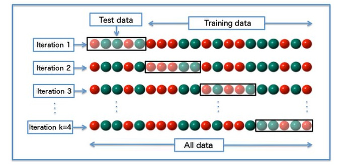
Figure 1.2 – K-fold cross-validation

Note

The preceding diagram has been reproduced according to the license specified: https://commons.wikimedia.org/wiki/File:K-fold_cross_validation.jpg.

For instance, let's choose k = 4 to match the illustration in Figure 1.2. The green and red balls correspond to the target class, where, in this case, we only have two target classes. The data is shuffled beforehand, which can be seen from the absence of a pattern of green and red balls. It is also worth mentioning that the shuffling was previously only done once. That's why the order of green and red balls is always the same for each iteration (fold). The black box in each fold corresponds to the validation set (the test data is in the illustration).

As you can see in Figure 1.2, the proportion of the training set versus the validation set is (k-1):1, or in this case, 3:1. During each fold, the model will be trained on the train set and evaluated on the validation set. Notice that the training and validation sets are different across each fold. The final evaluation score can be calculated by taking the average score of all of the folds.

In summary, k-fold cross-validation works as follows:

1. Shuffling the original full data
2. Holding out the test data
3. Performing the k-fold multiple evaluation strategy on the rest of the original full data
4. Calculating the final evaluation score by taking the average score of all of the folds
5. Evaluating the test data using the final model configuration

You might ask why do we need to perform cross-validation in the first place? Why is the vanilla train-validation-test splitting strategy not enough? There are several reasons why we need to apply the cross-validation strategy:

• Having only a small amount of training data.
• To get a more confident conclusion from the evaluation performance.
• To get a clearer picture of our model's learning ability and/or the complexity of the given data.

The first and second reasons are quite straightforward. The third reason is more interesting and should be discussed. How can cross-validation help us to get a better idea about our model's learning ability and/or the data complexity? Well, this happens when the variation of evaluation scores from each fold is quite big. For instance, out of 4 folds, we get accuracy scores of 45%, 82%, 64%, and 98%. This scenario should trigger our curiosity: what is wrong with our model and/or data? It could be that the data is too hard to learn and/or our model can't learn properly.

The following is the syntax to perform k-fold cross-validation via the Scikit-Learn package:

From sklearn.model_selection import train_test_split, Kfold
df_cv, df_test = train_test_split(df, test_size=0.2, random_state=0)
kf = Kfold(n_splits=4)
for train_index, val_index in kf.split(df_cv):
df_train, df_val = df_cv.iloc[train_index], df_cv.iloc[val_index]
#perform training or hyperparameter tuning here

Notice that, first, we hold out the test set and only work with df_cv when performing the k-fold cross-validation. By default, the Kfold function will disable the shuffling procedure. However, this is not a problem for us since the data has already shuffled beforehand when we called the train_test_split function. If you want to run the shuffling procedure again, you can pass shuffle=True in the Kfold function.

Here is another example if you are interested in learning how to apply the concept of stratifying splits in k-fold cross-validation:

From sklearn.model_selection import train_test_split, StratifiedKFold
df_cv, df_test = train_test_split(df, test_size=0.2, random_state=0, stratify=df['class'])
skf = StratifiedKFold(n_splits=4)
for train_index, val_index in skf.split(df_cv, df_cv['class']):
df_train, df_val = df_cv.iloc[train_index], df_cv.iloc[val_index]
#perform training or hyperparameter tuning here

The only difference is to import StratifiedKFold instead of the Kfold function and add the array of target variables, which will be used to split the data in a stratified fashion.

In this section, you have learned what cross-validation is, when the right time is to perform cross-validation, and the first (and the most widely used) cross-validation strategy variation, which is called k-fold cross-validation. In the subsequent sections, we will also learn other variations of cross-validation and how to implement them using the Scikit-Learn package.