

What is ML?
As the name suggests, ML generally refers to the area of computer science that involves making machines learn and make decisions on their own rather than acting on a set of explicit instructions. In this case, think about the machine as the processor of a computer and the instructions as a program written in a particular programming language. The compiler or the interpreter parses the program and derives a set of instructions that the processor can then execute. In this case, the programmer is responsible for making sure the logic they have in their program is correct as the processor will just perform the task as instructed.
For example, let’s assume you want to create a marketing campaign for a new product and want to target the right population to send the email to. To identify this population, you can create a rule in SQL to filter out the right population using a query. We can create rules around age, purchase history, gender, and so on and so forth, and will just process the inputs based on these rules. This is depicted in the following diagram.
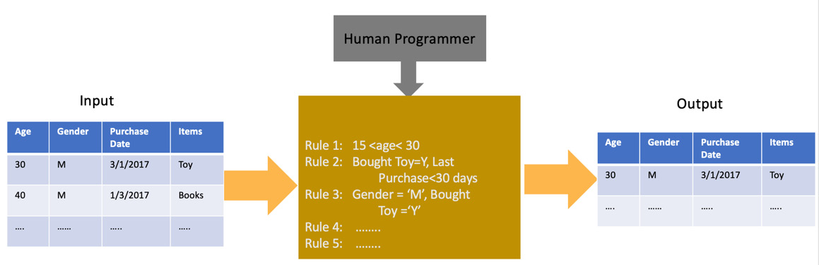
Figure 1.1 – A diagram showing the input, logic, and output of a traditional software program
In the case of ML, we allow the processor to “learn” from past data points about what is correct and incorrect. This process is called training. It then tries to apply that learning to unseen data points to make a decision. This process is known as prediction because it usually involves determining events that haven’t yet happened. We can represent the previous problem as an ML problem in the following way.
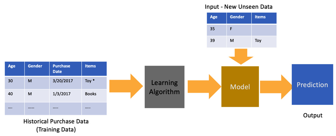
Figure 1.2 – A diagram showing how historical data is used to generate predictions using an ML model
As shown in the preceding diagram, we feed the learning algorithm with some known data points in the form of training data. The algorithm then comes up with a model that is now able to predict outputs from unseen data.
While ML models can be highly accurate, it is worth noting that the output of a model provides a probabilistic estimation of an answer instead of deterministic, like in the case of a software program. This means that ML models help us predict the probability of something happening, rather than telling us what will happen for sure. For this reason, it is important to continuously evaluate an ML model’s output and determine whether there is a need for it to be trained again.
Also, downstream consumers of an ML model (client applications) need to keep the probabilistic nature of the output in mind before making decisions based on it. For example, software to compute the sales numbers at the end of each quarter will provide a deterministic figure based on which you can calculate your profit for the quarter. However, an ML model will predict the sales number at the end of a future quarter, based on which you can predict what your profit would look like. The former can be entered in the books or ledger but the latter can be used to get an idea of the future result and take corrective actions if needed.
Now that we have a basic understanding of how to define ML as a concept, let’s look at two broad types of ML.
Supervised versus unsupervised learning
At a high level, ML models can be divided into two categories:
- Supervised learning model: A supervised ML model is created when the training data has a target variable in place. In other words, the training data contains unique combinations of input features and target variables. This is known as a labeled dataset. The supervised learning model learns the relationship between the target and the input features during the training process. Hence, it is important to have high-quality labeled datasets when training supervised learning models. Examples of supervised learning models include classification and regression models. Figure 1.3 depicts how this would work for a model that recognizes the breed of dogs.
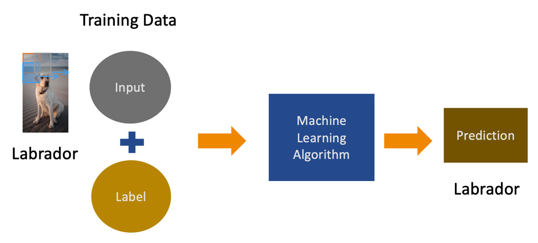
Figure 1.3 – A diagram showing a typical supervised learning prediction workflow
- Unsupervised learning model: An unsupervised learning model does not depend on the availability of labeled datasets. In other words, unlike its supervised cousin, the unsupervised learning model does not learn the association between the target variable and the input features. Instead, it learns the patterns in the overall data to determine how similar or different each data point is from the others. This is usually done by representing all the data points in parameter space in two or three dimensions and calculating the distance between them. The closer they are to each other, the more similar they are to each other. A common example of an unsupervised learning model is k-means clustering, which divides the input data points into k number of groups or clusters.

Figure 1.4 – A diagram showing a typical unsupervised learning prediction workflow
Now that we have an understanding of the two broad types of ML models, let us review a few key terms and concepts that are commonly used in ML.
ML terminology
There are some key concepts and terminologies specific to ML and it’s important to get a good understanding of these concepts before you go deeper into the subject. These terms will be used repeatedly throughout this book:
- Algorithm: Algorithms are at the core of an ML workflow. The algorithm defines how the training data is utilized to learn from its representations, and is then used to make predictions of a target variable. An example of an algorithm is linear regression. This algorithm is used to find the best fit line that minimizes the error between the actual and the predicted values of the target. This best fit line can be represented by a linear equation such as
y=ax+b. This type of algorithm can be used for problems that can be represented by linear relationships. For example, predicting the height of a person based on their age or predicting the cost of a house based on its square footage.
However, not all problems can be solved using a linear equation because the relationship between the target and the input data points might be non-linear, represented by a curve instead of a straight line. In the case of non-linear regression, the curve is represented by a nonlinear equation y=f(x,c)+b where f(x,c) can be any non-linear function. This type of algorithm can be used for problems that can be represented by non-linear relationships. For example, the prediction of the progression of a disease in a population can be driven by multiple non-linear relationships. An example of a non-linear algorithm is a decision tree. This algorithm aims to learn how to split the data into smaller subsets till the subset is as close in representation to the target variable as possible.
The choice of algorithm to solve a particular problem ultimately depends on multiple factors. It is often recommended to try multiple algorithms and find the one that works best for a particular problem. However, having an intuition of how the algorithm works allows you to narrow it down to a few.
- Training: Training is the process by which an algorithm learns. In other words, it helps converge on the best fit line or curve based on the input dataset and the target variable. As a result, it is also sometimes referred to as fitting. During the training process, the input data and the target are fed into the algorithm iteratively, in batches. The process tries to determine the coefficients of the final equation that represents the line or the curve with the minimum error when compared to the target variable. During the training process, the input dataset is divided into three different groups: train, validation, and test. The train dataset is the majority of the input data and is used to fit or train the model. The validation dataset is used to evaluate the model performance and, if necessary, tune the model input parameters (also known as hyperparameters) in an iterative way. Finally, the test dataset is the dataset on which the final evaluation of the model is done, which determines whether it can be deployed in production. The process of training and tuning the model is highly iterative. It requires multiple runs and trial and error to determine the best combination of parameters to use in the final model.
The evaluation of the ML model is done by a metric, also known as the evaluation metric, which determines how good the model is. Depending on the choice of the evaluation metric, the training process aims to minimize or maximize the value of the metric. For instance, if the evaluation metric is Mean Squared Error, the goal of the training job is to minimize it. However, if the evaluation metric is accuracy, the goal would be to maximize it. Training is a compute-intensive process and can consume considerable resources.
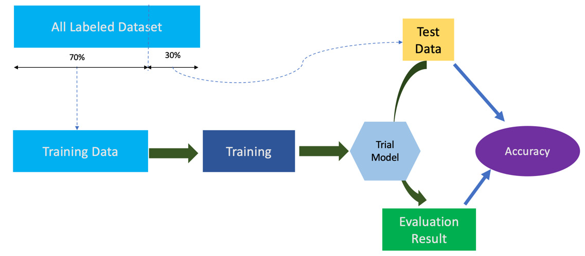
Figure 1.5 – A diagram showing the steps of a model training workflow
- Model: An ML model is an artifact that results from the training process. In essence, when you train an algorithm with data, it results in a model. A model accepts input parameters and provides the predicted value of the target variable. The input parameters should be exactly the same in structure and format as the training data input parameters. The model can be serialized into a format that can be stored as a file and then deployed into a workflow to generate predictions. The serialized model file stores the weights or coefficients that, when applied to the equation, result in the value of the predicted target. To generate predictions, the model needs to be de-serialized or reconstructed from the saved model file. The idea of saving the model to the disk by serializing it allows for model portability, a term typically used by data scientists to denote interchangeability between frameworks when it comes to data science. Common ML frameworks such as PyTorch, scikit-learn, and TensorFlow all support serializing model files into standard formats, which allows you to standardize your model registries and also use them interchangeably if needed.
- Inference: Inference is the process of generating predictions from the trained model. Hence, this step is also known as predicting. The model that has been trained on past data is now exposed to unseen data to generate the value of the target variable. As described earlier, the model resulting from the training process is already evaluated using a metric on a test dataset, which is a subset of the input data. However, this does not guarantee that the model will perform well on unseen data when deployed. As a result, prediction results are continuously monitored and compared against the ground truth (actual) values.
There are various ways in which the model results are monitored and evaluated in production. One common method utilizes humans to evaluate certain prediction results that are suspicious. This method of validation is also known as human-in-the-loop. In this method, the model results with lower confidence (usually denoted by a confidence score) are routed to a human to determine if the output is correct or not. The human can then override the model result if needed before sending it to the downstream system. This method, while extremely useful, has a drawback. Some ML models do not have the ground truth data available until the event actually happens in the future. For instance, if the model predicts a patient is going to require a kidney transplant, a human may not be able to validate that output of the model until the transplant actually happens (or not). In such cases, the human-in-the-loop method of validation does not work. To account for such limitations, the method of monitoring drift in real-world data compared to the training data is utilized to determine the effectiveness of the model predictions. If the real-world data is very different from the training data, the chances of predictions being correct are minimal and hence, it may require retraining the model.
Inferences from an ML model can be executed as an asynchronous batch process or as a synchronous real-time process. An asynchronous process is great for workloads that run in batches. For example, calculating the risk score of loan defaults across all monthly loan applications at the end of the month. This risk score is generated or updated once a month for a large batch of individuals who applied for a loan. As a result, the model does not need to serve requests 24/7 and is only used at scheduled times. Synchronous or real-time inference is when the model serves out inference as a response to each request 24/7 in real time. In this case, the model needs to be hosted on a highly available infrastructure that remains up and running at all times and also adheres to the latency requirements of the downstream application. For example, a weather forecast application that continuously updates the forecast conditions based on the predictions from a model needs to generate predictions 24/7 in real time.
Now that we have a good understanding of what ML is and the key terminologies associated with it, let’s look at the process of building the model in more detail.