-
Book Overview & Buying

-
Table Of Contents

Data Labeling in Machine Learning with Python
By :
Data Labeling in Machine Learning with Python
By:
Overview of this book
Data labeling is the invisible hand that guides the power of artificial intelligence and machine learning. In today’s data-driven world, mastering data labeling is not just an advantage, it’s a necessity. Data Labeling in Machine Learning with Python empowers you to unearth value from raw data, create intelligent systems, and influence the course of technological evolution.
With this book, you'll discover the art of employing summary statistics, weak supervision, programmatic rules, and heuristics to assign labels to unlabeled training data programmatically. As you progress, you'll be able to enhance your datasets by mastering the intricacies of semi-supervised learning and data augmentation. Venturing further into the data landscape, you'll immerse yourself in the annotation of image, video, and audio data, harnessing the power of Python libraries such as seaborn, matplotlib, cv2, librosa, openai, and langchain. With hands-on guidance and practical examples, you'll gain proficiency in annotating diverse data types effectively.
By the end of this book, you’ll have the practical expertise to programmatically label diverse data types and enhance datasets, unlocking the full potential of your data.
Table of Contents (18 chapters)
Preface

Part 1: Labeling Tabular Data
 Free Chapter
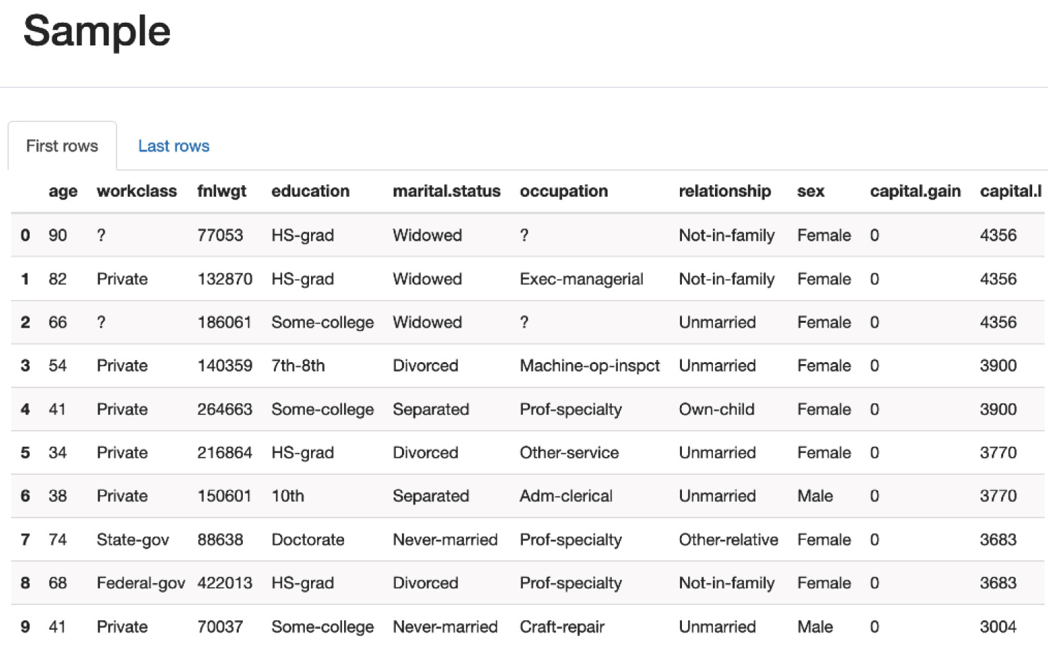
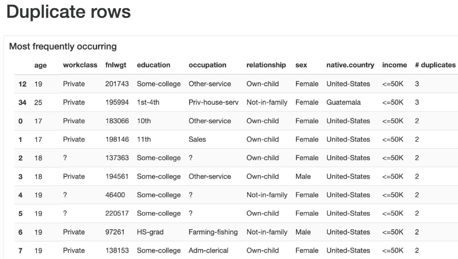
Chapter 1: Exploring Data for Machine Learning
Chapter 2: Labeling Data for Classification
Chapter 3: Labeling Data for Regression
Part 2: Labeling Image Data
Chapter 4: Exploring Image Data
Chapter 5: Labeling Image Data Using Rules
Chapter 6: Labeling Image Data Using Data Augmentation
Part 3: Labeling Text, Audio, and Video Data
Chapter 7: Labeling Text Data
Chapter 8: Exploring Video Data
Chapter 9: Labeling Video Data
Chapter 10: Exploring Audio Data
Chapter 11: Labeling Audio Data
Chapter 12: Hands-On Exploring Data Labeling Tools
Index