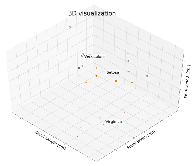
In this section, we will explore a basic one-shot learning approach. As humans, we have a hierarchical way of thinking. For example, if we see something unknown to us, we look for its similarity to objects we already know. Similarly, in this exercise, we will use a nonparametric kNN approach to find classes. We will also compare its performance to the basic neural network architecture.

In this exercise, we will compare kNN to neural networks where we have a small dataset. We will be using the iris dataset imported from the scikit-learn library.

To begin, we will first discuss the basics of kNN. The kNN classifier is a nonparametric classifier that simply stores the training data, D, and classifies each new instance using a majority vote over its set of k nearest neighbors, computed using any distance function. For a kNN, we need to choose the distance function, d, and the number of neighbors, k:

Follow these steps to compare kNN with a neural network:

1. Import all the libraries required for this exercise using the following code:

import numpy as np
import matplotlib.pyplot as plt
from sklearn import datasets
from sklearn.neighbors import KNeighborsClassifier
from sklearn.model_selection import train_test_split
from sklearn.metrics import confusion_matrix, accuracy_score
from sklearn.model_selection import cross_val_score
from sklearn.neural_network import MLPClassifier

2. Import the iris dataset:

# import small dataset
iris = datasets.load_iris()
X = iris.data
y = iris.target

3. To ensure we are using a very small dataset, we will randomly choose 30 points and print them using the following code:

indices=np.random.choice(len(X), 30)
X=X[indices]
y=y[indices]
print (y)

This will be the resultant output:

[2 1 2 1 2 0 1 0 0 0 2 1 1 0 0 0 2 2 1 2 1 0 0 1 2 0 0 2 0 0]

4. To understand our features, we will try to plot them in 3D as a scatterplot:

from mpl_toolkits.mplot3d import Axes3D
fig = plt.figure(1, figsize=(20, 15))
ax = Axes3D(fig, elev=48, azim=134)
ax.scatter(X[:, 0], X[:, 1], X[:, 2], c=y,
         cmap=plt.cm.Set1, edgecolor='k', s = X[:, 3]*50)

for name, label in [('Virginica', 0), ('Setosa', 1), ('Versicolour', 2)]:
    ax.text3D(X[y == label, 0].mean(),
              X[y == label, 1].mean(),
              X[y == label, 2].mean(), name,
              horizontalalignment='center',
              bbox=dict(alpha=.5, edgecolor='w', facecolor='w'),size=25)

ax.set_title("3D visualization", fontsize=40)
ax.set_xlabel("Sepal Length [cm]", fontsize=25)
ax.w_xaxis.set_ticklabels([])
ax.set_ylabel("Sepal Width [cm]", fontsize=25)
ax.w_yaxis.set_ticklabels([])
ax.set_zlabel("Petal Length [cm]", fontsize=25)
ax.w_zaxis.set_ticklabels([])

plt.show()

The following plot is the output. As we can see in the 3D visualization, data points are usually found in groups:

5. To begin with, we will first split the dataset into training and testing sets using an 80:20 split. We will be using k=3 as the nearest neighbor:

X_train, X_test, y_train, y_test = train_test_split(X, y, test_size = 0.2, random_state = 0)
# Instantiate learning model (k = 3)
classifier = KNeighborsClassifier(n_neighbors=3)

# Fitting the model
classifier.fit(X_train, y_train)

# Predicting the Test set results
y_pred = classifier.predict(X_test)

cm = confusion_matrix(y_test, y_pred)

accuracy = accuracy_score(y_test, y_pred)*100
print('Accuracy of our model is equal ' + str(round(accuracy, 2)) + ' %.')

This will result in the following output:

Accuracy of our model is equal 83.33 %.

6. Initialize the hidden layers' sizes and the number of iterations:

mlp = MLPClassifier(hidden_layer_sizes=(13,13,13),max_iter=10)
mlp.fit(X_train,y_train)

7. We will predict our test dataset for both kNN and a neural network and then compare the two:

predictions = mlp.predict(X_test)

accuracy = accuracy_score(y_test, predictions)*100
print('Accuracy of our model is equal ' + str(round(accuracy, 2)) + ' %.')

The following is the resultant output:

Accuracy of our model is equal 50.0 %.

For our current scenario, we can see that the neural network is less accurate than the kNN. This could be due to a lot of reasons, including the randomness of the dataset, the choice of neighbors, and the number of layers. But if we run it enough times, we will observe that a kNN is more likely to give a better output as it always stores data points, instead of learning parameters as neural networks do. Therefore, a kNN can be called a one-shot learning method.