

"Data! Data! Data!" he cried impatiently. "I can't make bricks without clay." | ||
| --Sherlock Holmes - The Adventure of the Copper Beeches | ||
Everything you do with a computer is managing data. Data comes in many different shapes and flavors. It's the music you listen, the movie you stream, the PDFs you open. Even the chapter you're reading at this very moment is just a file, which is data.
Data can be simple, an integer number to represent an age, or complex, like an order placed on a website. It can be about a single object or about a collection of them.
Data can even be about data, that is, metadata. Data that describes the design of other data structures or data that describes application data or its context.
In Python, objects are abstraction for data, and Python has an amazing variety of data structures that you can use to represent data, or combine them to create your own custom data. Before we delve into the specifics, I want you to be very clear about objects in Python, so let's talk a little bit more about them.
As we already said, everything in Python is an object. But what really happens when you type an instruction like age = 42 in a Python module?
Tip
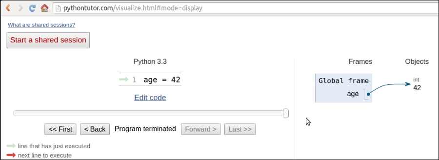
If you go to http://pythontutor.com/, you can type that instruction into a text box and get its visual representation. Keep this website in mind, it's very useful to consolidate your understanding of what goes on behind the scenes.
So, what happens is that an object is created. It gets an id, the type is set to int (integer number), and the value to 42. A name age is placed in the global namespace, pointing to that object. Therefore, whenever we are in the global namespace, after the execution of that line, we can retrieve that object by simply accessing it through its name: age.
If you were to move house, you would put all the knives, forks, and spoons in a box and label it cutlery. Can you see it's exactly the same concept? Here's a screenshot of how it may look like (you may have to tweak the settings to get to the same view):
So, for the rest of this chapter, whenever you read something such as name = some_value, think of a name placed in the namespace that is tied to the scope in which the instruction was written, with a nice arrow pointing to an object that has an id, a type, and a value. There is a little bit more to say about this mechanism, but it's much easier to talk about it over an example, so we'll get back to this later.
A first fundamental distinction that Python makes on data is about whether or not the value of an object changes. If the value can change, the object is called mutable, while if the value cannot change, the object is called immutable.
It is very important that you understand the distinction between mutable and immutable because it affects the code you write, so here's a question:
>>> age = 42 >>> age 42 >>> age = 43 #A >>> age 43
In the preceding code, on the line #A, have I changed the value of age? Well, no. But now it's 43 (I hear you say...). Yes, it's 43, but 42 was an integer number, of the type int, which is immutable. So, what happened is really that on the first line, age is a name that is set to point to an int object, whose value is 42. When we type age = 43, what happens is that another object is created, of the type int and value 43 (also, the id will be different), and the name age is set to point to it. So, we didn't change that 42 to 43. We actually just pointed age to a different location: the new int object whose value is 43. Let's see the same code also printing the IDs:
>>> age = 42 >>> id(age) 10456352 >>> age = 43 >>> id(age) 10456384
Notice that we print the IDs by calling the built-in id function. As you can see, they are different, as expected. Bear in mind that age points to one object at a time: 42 first, then 43. Never together.
Now, let's see the same example using a mutable object. For this example, let's just use a Person object, that has a property age:
>>> fab = Person(age=39) >>> fab.age 39 >>> id(fab) 139632387887456 >>> fab.age = 29 # I wish! >>> id(fab) 139632387887456 # still the same id
In this case, I set up an object fab whose type is Person (a custom class). On creation, the object is given the age of 39. I'm printing it, along with the object id, right afterwards. Notice that, even after I change age to be 29, the ID of fab stays the same (while the ID of age has changed, of course). Custom objects in Python are mutable (unless you code them not to be). Keep this concept in mind, it's very important. I'll remind you about it through the rest of the chapter.
Let's start by exploring Python's built-in data types for numbers. Python was designed by a man with a master's degree in mathematics and computer science, so it's only logical that it has amazing support for numbers.
Numbers are immutable objects.
Python integers have unlimited range, subject only to the available virtual memory. This means that it doesn't really matter how big a number you want to store: as long as it can fit in your computer's memory, Python will take care of it. Integer numbers can be positive, negative, and 0 (zero). They support all the basic mathematical operations, as shown in the following example:
>>> a = 12 >>> b = 3 >>> a + b # addition 15 >>> b - a # subtraction -9 >>> a // b # integer division 4 >>> a / b # true division 4.0 >>> a * b # multiplication 36 >>> b ** a # power operator 531441 >>> 2 ** 1024 # a very big number, Python handles it gracefully 17976931348623159077293051907890247336179769789423065727343008115 77326758055009631327084773224075360211201138798713933576587897688 14416622492847430639474124377767893424865485276302219601246094119 45308295208500576883815068234246288147391311054082723716335051068 4586298239947245938479716304835356329624224137216
The preceding code should be easy to understand. Just notice one important thing: Python has two division operators, one performs the so-called true division (/), which returns the quotient of the operands, and the other one, the so-called integer division (//), which returns the floored quotient of the operands. See how that is different for positive and negative numbers:
>>> 7 / 4 # true division 1.75 >>> 7 // 4 # integer division, flooring returns 1 1 >>> -7 / 4 # true division again, result is opposite of previous -1.75 >>> -7 // 4 # integer div., result not the opposite of previous -2
This is an interesting example. If you were expecting a -1 on the last line, don't feel bad, it's just the way Python works. The result of an integer division in Python is always rounded towards minus infinity. If instead of flooring you want to truncate a number to an integer, you can use the built-in int function, like shown in the following example:
>>> int(1.75) 1 >>> int(-1.75) -1
Notice that truncation is done towards 0.
There is also an operator to calculate the remainder of a division. It's called modulo operator, and it's represented by a percent (%):
>>> 10 % 3 # remainder of the division 10 // 3 1 >>> 10 % 4 # remainder of the division 10 // 4 2
Boolean algebra is that subset of algebra in which the values of the variables are the truth values: true and false. In Python, True and False are two keywords that are used to represent truth values. Booleans are a subclass of integers, and behave respectively like 1 and 0. The equivalent of the int class for Booleans is the bool class, which returns either True or False. Every built-in Python object has a value in the Boolean context, which means they basically evaluate to either True or False when fed to the bool function. We'll see all about this in Chapter 3, Iterating and Making Decisions.
Boolean values can be combined in Boolean expressions using the logical operators and, or, and not. Again, we'll see them in full in the next chapter, so for now let's just see a simple example:
>>> int(True) # True behaves like 1 1 >>> int(False) # False behaves like 0 0 >>> bool(1) # 1 evaluates to True in a boolean context True >>> bool(-42) # and so does every non-zero number True >>> bool(0) # 0 evaluates to False False >>> # quick peak at the operators (and, or, not) >>> not True False >>> not False True >>> True and True True >>> False or True True
You can see that True and False are subclasses of integers when you try to add them. Python upcasts them to integers and performs addition:
>>> 1 + True 2 >>> False + 42 42 >>> 7 - True 6
Note
Upcasting is a type conversion operation that goes from a subclass to its parent. In the example presented here, True and False, which belong to a class derived from the integer class, are converted back to integers when needed. This topic is about inheritance and will be explained in detail in Chapter 6, Advanced Concepts – OOP, Decorators, and Iterators.
Real numbers, or floating point numbers, are represented in Python according to the IEEE 754 double-precision binary floating-point format, which is stored in 64 bits of information divided into three sections: sign, exponent, and mantissa.
Note
Quench your thirst for knowledge about this format on Wikipedia: http://en.wikipedia.org/wiki/Double-precision_floating-point_format
Usually programming languages give coders two different formats: single and double precision. The former taking up 32 bits of memory, and the latter 64. Python supports only the double format. Let's see a simple example:
>>> pi = 3.1415926536 # how many digits of PI can you remember? >>> radius = 4.5 >>> area = pi * (radius ** 2) >>> area 63.61725123519331
The sys.float_info struct sequence holds information about how floating point numbers will behave on your system. This is what I see on my box:
>>> import sys >>> sys.float_info sys.float_info(max=1.7976931348623157e+308, max_exp=1024, max_10_exp=308, min=2.2250738585072014e-308, min_exp=-1021, min_10_exp=-307, dig=15, mant_dig=53, epsilon=2.220446049250313e-16, radix=2, rounds=1)
Let's make a few considerations here: we have 64 bits to represent float numbers. This means we can represent at most 2 ** 64 == 18,446,744,073,709,551,616 numbers with that amount of bits. Take a look at the max and epsilon value for the float numbers, and you'll realize it's impossible to represent them all. There is just not enough space so they are approximated to the closest representable number. You probably think that only extremely big or extremely small numbers suffer from this issue. Well, think again:
>>> 3 * 0.1 – 0.3 # this should be 0!!! 5.551115123125783e-17
What does this tell you? It tells you that double precision numbers suffer from approximation issues even when it comes to simple numbers like 0.1 or 0.3. Why is this important? It can be a big problem if you're handling prices, or financial calculations, or any kind of data that needs not to be approximated. Don't worry, Python gives you the Decimal type, which doesn't suffer from these issues, we'll see them in a bit.
Python gives you complex numbers support out of the box. If you don't know what complex numbers are, you can look them up on the Web. They are numbers that can be expressed in the form a + ib where a and b are real numbers, and i (or j if you're an engineer) is the imaginary unit, that is, the square root of -1. a and b are called respectively the real and imaginary part of the number.
It's actually unlikely you'll be using them, unless you're coding something scientific. Let's see a small example:
>>> c = 3.14 + 2.73j >>> c.real # real part 3.14 >>> c.imag # imaginary part 2.73 >>> c.conjugate() # conjugate of A + Bj is A - Bj (3.14-2.73j) >>> c * 2 # multiplication is allowed (6.28+5.46j) >>> c ** 2 # power operation as well (2.4067000000000007+17.1444j) >>> d = 1 + 1j # addition and subtraction as well >>> c - d (2.14+1.73j)
Let's finish the tour of the number department with a look at fractions and decimals. Fractions hold a rational numerator and denominator in their lowest forms. Let's see a quick example:
>>> from fractions import Fraction >>> Fraction(10, 6) # mad hatter? Fraction(5, 3) # notice it's been reduced to lowest terms >>> Fraction(1, 3) + Fraction(2, 3) # 1/3 + 2/3 = 3/3 = 1/1 Fraction(1, 1) >>> f = Fraction(10, 6) >>> f.numerator 5 >>> f.denominator 3
Although they can be very useful at times, it's not that common to spot them in commercial software. Much easier instead, is to see decimal numbers being used in all those contexts where precision is everything, for example, scientific and financial calculations.
Note
It's important to remember that arbitrary precision decimal numbers come at a price in performance, of course. The amount of data to be stored for each number is far greater than it is for fractions or floats as well as the way they are handled, which requires the Python interpreter much more work behind the scenes. Another interesting thing to know is that you can get and set the precision by accessing decimal.getcontext().prec.
Let's see a quick example with Decimal numbers:
>>> from decimal import Decimal as D # rename for brevity >>> D(3.14) # pi, from float, so approximation issues Decimal('3.140000000000000124344978758017532527446746826171875') >>> D('3.14') # pi, from a string, so no approximation issues Decimal('3.14') >>> D(0.1) * D(3) - D(0.3) # from float, we still have the issue Decimal('2.775557561565156540423631668E-17') >>> D('0.1') * D(3) - D('0.3') # from string, all perfect Decimal('0.0')
Notice that when we construct a Decimal number from a float, it takes on all the approximation issues the float may come from. On the other hand, when the Decimal has no approximation issues, for example, when we feed an int or a string representation to the constructor, then the calculation has no quirky behavior. When it comes to money, use decimals.
This concludes our introduction to built-in numeric types, let's now see sequences.
Integers
Python integers have unlimited range, subject only to the available virtual memory. This means that it doesn't really matter how big a number you want to store: as long as it can fit in your computer's memory, Python will take care of it. Integer numbers can be positive, negative, and 0 (zero). They support all the basic mathematical operations, as shown in the following example:
>>> a = 12 >>> b = 3 >>> a + b # addition 15 >>> b - a # subtraction -9 >>> a // b # integer division 4 >>> a / b # true division 4.0 >>> a * b # multiplication 36 >>> b ** a # power operator 531441 >>> 2 ** 1024 # a very big number, Python handles it gracefully 17976931348623159077293051907890247336179769789423065727343008115 77326758055009631327084773224075360211201138798713933576587897688 14416622492847430639474124377767893424865485276302219601246094119 45308295208500576883815068234246288147391311054082723716335051068 4586298239947245938479716304835356329624224137216
The preceding code should be easy to understand. Just notice one important thing: Python has two division operators, one performs the so-called true division (/), which returns the quotient of the operands, and the other one, the so-called integer division (//), which returns the floored quotient of the operands. See how that is different for positive and negative numbers:
>>> 7 / 4 # true division 1.75 >>> 7 // 4 # integer division, flooring returns 1 1 >>> -7 / 4 # true division again, result is opposite of previous -1.75 >>> -7 // 4 # integer div., result not the opposite of previous -2
This is an interesting example. If you were expecting a -1 on the last line, don't feel bad, it's just the way Python works. The result of an integer division in Python is always rounded towards minus infinity. If instead of flooring you want to truncate a number to an integer, you can use the built-in int function, like shown in the following example:
>>> int(1.75) 1 >>> int(-1.75) -1
Notice that truncation is done towards 0.
There is also an operator to calculate the remainder of a division. It's called modulo operator, and it's represented by a percent (%):
>>> 10 % 3 # remainder of the division 10 // 3 1 >>> 10 % 4 # remainder of the division 10 // 4 2
Boolean algebra is that subset of algebra in which the values of the variables are the truth values: true and false. In Python, True and False are two keywords that are used to represent truth values. Booleans are a subclass of integers, and behave respectively like 1 and 0. The equivalent of the int class for Booleans is the bool class, which returns either True or False. Every built-in Python object has a value in the Boolean context, which means they basically evaluate to either True or False when fed to the bool function. We'll see all about this in Chapter 3, Iterating and Making Decisions.
Boolean values can be combined in Boolean expressions using the logical operators and, or, and not. Again, we'll see them in full in the next chapter, so for now let's just see a simple example:
>>> int(True) # True behaves like 1 1 >>> int(False) # False behaves like 0 0 >>> bool(1) # 1 evaluates to True in a boolean context True >>> bool(-42) # and so does every non-zero number True >>> bool(0) # 0 evaluates to False False >>> # quick peak at the operators (and, or, not) >>> not True False >>> not False True >>> True and True True >>> False or True True
You can see that True and False are subclasses of integers when you try to add them. Python upcasts them to integers and performs addition:
>>> 1 + True 2 >>> False + 42 42 >>> 7 - True 6
Note
Upcasting is a type conversion operation that goes from a subclass to its parent. In the example presented here, True and False, which belong to a class derived from the integer class, are converted back to integers when needed. This topic is about inheritance and will be explained in detail in Chapter 6, Advanced Concepts – OOP, Decorators, and Iterators.
Real numbers, or floating point numbers, are represented in Python according to the IEEE 754 double-precision binary floating-point format, which is stored in 64 bits of information divided into three sections: sign, exponent, and mantissa.
Note
Quench your thirst for knowledge about this format on Wikipedia: http://en.wikipedia.org/wiki/Double-precision_floating-point_format
Usually programming languages give coders two different formats: single and double precision. The former taking up 32 bits of memory, and the latter 64. Python supports only the double format. Let's see a simple example:
>>> pi = 3.1415926536 # how many digits of PI can you remember? >>> radius = 4.5 >>> area = pi * (radius ** 2) >>> area 63.61725123519331
The sys.float_info struct sequence holds information about how floating point numbers will behave on your system. This is what I see on my box:
>>> import sys >>> sys.float_info sys.float_info(max=1.7976931348623157e+308, max_exp=1024, max_10_exp=308, min=2.2250738585072014e-308, min_exp=-1021, min_10_exp=-307, dig=15, mant_dig=53, epsilon=2.220446049250313e-16, radix=2, rounds=1)
Let's make a few considerations here: we have 64 bits to represent float numbers. This means we can represent at most 2 ** 64 == 18,446,744,073,709,551,616 numbers with that amount of bits. Take a look at the max and epsilon value for the float numbers, and you'll realize it's impossible to represent them all. There is just not enough space so they are approximated to the closest representable number. You probably think that only extremely big or extremely small numbers suffer from this issue. Well, think again:
>>> 3 * 0.1 – 0.3 # this should be 0!!! 5.551115123125783e-17
What does this tell you? It tells you that double precision numbers suffer from approximation issues even when it comes to simple numbers like 0.1 or 0.3. Why is this important? It can be a big problem if you're handling prices, or financial calculations, or any kind of data that needs not to be approximated. Don't worry, Python gives you the Decimal type, which doesn't suffer from these issues, we'll see them in a bit.
Python gives you complex numbers support out of the box. If you don't know what complex numbers are, you can look them up on the Web. They are numbers that can be expressed in the form a + ib where a and b are real numbers, and i (or j if you're an engineer) is the imaginary unit, that is, the square root of -1. a and b are called respectively the real and imaginary part of the number.
It's actually unlikely you'll be using them, unless you're coding something scientific. Let's see a small example:
>>> c = 3.14 + 2.73j >>> c.real # real part 3.14 >>> c.imag # imaginary part 2.73 >>> c.conjugate() # conjugate of A + Bj is A - Bj (3.14-2.73j) >>> c * 2 # multiplication is allowed (6.28+5.46j) >>> c ** 2 # power operation as well (2.4067000000000007+17.1444j) >>> d = 1 + 1j # addition and subtraction as well >>> c - d (2.14+1.73j)
Let's finish the tour of the number department with a look at fractions and decimals. Fractions hold a rational numerator and denominator in their lowest forms. Let's see a quick example:
>>> from fractions import Fraction >>> Fraction(10, 6) # mad hatter? Fraction(5, 3) # notice it's been reduced to lowest terms >>> Fraction(1, 3) + Fraction(2, 3) # 1/3 + 2/3 = 3/3 = 1/1 Fraction(1, 1) >>> f = Fraction(10, 6) >>> f.numerator 5 >>> f.denominator 3
Although they can be very useful at times, it's not that common to spot them in commercial software. Much easier instead, is to see decimal numbers being used in all those contexts where precision is everything, for example, scientific and financial calculations.
Note
It's important to remember that arbitrary precision decimal numbers come at a price in performance, of course. The amount of data to be stored for each number is far greater than it is for fractions or floats as well as the way they are handled, which requires the Python interpreter much more work behind the scenes. Another interesting thing to know is that you can get and set the precision by accessing decimal.getcontext().prec.
Let's see a quick example with Decimal numbers:
>>> from decimal import Decimal as D # rename for brevity >>> D(3.14) # pi, from float, so approximation issues Decimal('3.140000000000000124344978758017532527446746826171875') >>> D('3.14') # pi, from a string, so no approximation issues Decimal('3.14') >>> D(0.1) * D(3) - D(0.3) # from float, we still have the issue Decimal('2.775557561565156540423631668E-17') >>> D('0.1') * D(3) - D('0.3') # from string, all perfect Decimal('0.0')
Notice that when we construct a Decimal number from a float, it takes on all the approximation issues the float may come from. On the other hand, when the Decimal has no approximation issues, for example, when we feed an int or a string representation to the constructor, then the calculation has no quirky behavior. When it comes to money, use decimals.
This concludes our introduction to built-in numeric types, let's now see sequences.
Booleans
Boolean algebra is that subset of algebra in which the values of the variables are the truth values: true and false. In Python, True and False are two keywords that are used to represent truth values. Booleans are a subclass of integers, and behave respectively like 1 and 0. The equivalent of the int class for Booleans is the bool class, which returns either True or False. Every built-in Python object has a value in the Boolean context, which means they basically evaluate to either True or False when fed to the bool function. We'll see all about this in Chapter 3, Iterating and Making Decisions.
Boolean values can be combined in Boolean expressions using the logical operators and, or, and not. Again, we'll see them in full in the next chapter, so for now let's just see a simple example:
>>> int(True) # True behaves like 1 1 >>> int(False) # False behaves like 0 0 >>> bool(1) # 1 evaluates to True in a boolean context True >>> bool(-42) # and so does every non-zero number True >>> bool(0) # 0 evaluates to False False >>> # quick peak at the operators (and, or, not) >>> not True False >>> not False True >>> True and True True >>> False or True True
You can see that True and False are subclasses of integers when you try to add them. Python upcasts them to integers and performs addition:
>>> 1 + True 2 >>> False + 42 42 >>> 7 - True 6
Note
Upcasting is a type conversion operation that goes from a subclass to its parent. In the example presented here, True and False, which belong to a class derived from the integer class, are converted back to integers when needed. This topic is about inheritance and will be explained in detail in Chapter 6, Advanced Concepts – OOP, Decorators, and Iterators.
Real numbers, or floating point numbers, are represented in Python according to the IEEE 754 double-precision binary floating-point format, which is stored in 64 bits of information divided into three sections: sign, exponent, and mantissa.
Note
Quench your thirst for knowledge about this format on Wikipedia: http://en.wikipedia.org/wiki/Double-precision_floating-point_format
Usually programming languages give coders two different formats: single and double precision. The former taking up 32 bits of memory, and the latter 64. Python supports only the double format. Let's see a simple example:
>>> pi = 3.1415926536 # how many digits of PI can you remember? >>> radius = 4.5 >>> area = pi * (radius ** 2) >>> area 63.61725123519331
The sys.float_info struct sequence holds information about how floating point numbers will behave on your system. This is what I see on my box:
>>> import sys >>> sys.float_info sys.float_info(max=1.7976931348623157e+308, max_exp=1024, max_10_exp=308, min=2.2250738585072014e-308, min_exp=-1021, min_10_exp=-307, dig=15, mant_dig=53, epsilon=2.220446049250313e-16, radix=2, rounds=1)
Let's make a few considerations here: we have 64 bits to represent float numbers. This means we can represent at most 2 ** 64 == 18,446,744,073,709,551,616 numbers with that amount of bits. Take a look at the max and epsilon value for the float numbers, and you'll realize it's impossible to represent them all. There is just not enough space so they are approximated to the closest representable number. You probably think that only extremely big or extremely small numbers suffer from this issue. Well, think again:
>>> 3 * 0.1 – 0.3 # this should be 0!!! 5.551115123125783e-17
What does this tell you? It tells you that double precision numbers suffer from approximation issues even when it comes to simple numbers like 0.1 or 0.3. Why is this important? It can be a big problem if you're handling prices, or financial calculations, or any kind of data that needs not to be approximated. Don't worry, Python gives you the Decimal type, which doesn't suffer from these issues, we'll see them in a bit.
Python gives you complex numbers support out of the box. If you don't know what complex numbers are, you can look them up on the Web. They are numbers that can be expressed in the form a + ib where a and b are real numbers, and i (or j if you're an engineer) is the imaginary unit, that is, the square root of -1. a and b are called respectively the real and imaginary part of the number.
It's actually unlikely you'll be using them, unless you're coding something scientific. Let's see a small example:
>>> c = 3.14 + 2.73j >>> c.real # real part 3.14 >>> c.imag # imaginary part 2.73 >>> c.conjugate() # conjugate of A + Bj is A - Bj (3.14-2.73j) >>> c * 2 # multiplication is allowed (6.28+5.46j) >>> c ** 2 # power operation as well (2.4067000000000007+17.1444j) >>> d = 1 + 1j # addition and subtraction as well >>> c - d (2.14+1.73j)
Let's finish the tour of the number department with a look at fractions and decimals. Fractions hold a rational numerator and denominator in their lowest forms. Let's see a quick example:
>>> from fractions import Fraction >>> Fraction(10, 6) # mad hatter? Fraction(5, 3) # notice it's been reduced to lowest terms >>> Fraction(1, 3) + Fraction(2, 3) # 1/3 + 2/3 = 3/3 = 1/1 Fraction(1, 1) >>> f = Fraction(10, 6) >>> f.numerator 5 >>> f.denominator 3
Although they can be very useful at times, it's not that common to spot them in commercial software. Much easier instead, is to see decimal numbers being used in all those contexts where precision is everything, for example, scientific and financial calculations.
Note
It's important to remember that arbitrary precision decimal numbers come at a price in performance, of course. The amount of data to be stored for each number is far greater than it is for fractions or floats as well as the way they are handled, which requires the Python interpreter much more work behind the scenes. Another interesting thing to know is that you can get and set the precision by accessing decimal.getcontext().prec.
Let's see a quick example with Decimal numbers:
>>> from decimal import Decimal as D # rename for brevity >>> D(3.14) # pi, from float, so approximation issues Decimal('3.140000000000000124344978758017532527446746826171875') >>> D('3.14') # pi, from a string, so no approximation issues Decimal('3.14') >>> D(0.1) * D(3) - D(0.3) # from float, we still have the issue Decimal('2.775557561565156540423631668E-17') >>> D('0.1') * D(3) - D('0.3') # from string, all perfect Decimal('0.0')
Notice that when we construct a Decimal number from a float, it takes on all the approximation issues the float may come from. On the other hand, when the Decimal has no approximation issues, for example, when we feed an int or a string representation to the constructor, then the calculation has no quirky behavior. When it comes to money, use decimals.
This concludes our introduction to built-in numeric types, let's now see sequences.
Reals
Real numbers, or floating point numbers, are represented in Python according to the IEEE 754 double-precision binary floating-point format, which is stored in 64 bits of information divided into three sections: sign, exponent, and mantissa.
Note
Quench your thirst for knowledge about this format on Wikipedia: http://en.wikipedia.org/wiki/Double-precision_floating-point_format
Usually programming languages give coders two different formats: single and double precision. The former taking up 32 bits of memory, and the latter 64. Python supports only the double format. Let's see a simple example:
>>> pi = 3.1415926536 # how many digits of PI can you remember? >>> radius = 4.5 >>> area = pi * (radius ** 2) >>> area 63.61725123519331
The sys.float_info struct sequence holds information about how floating point numbers will behave on your system. This is what I see on my box:
>>> import sys >>> sys.float_info sys.float_info(max=1.7976931348623157e+308, max_exp=1024, max_10_exp=308, min=2.2250738585072014e-308, min_exp=-1021, min_10_exp=-307, dig=15, mant_dig=53, epsilon=2.220446049250313e-16, radix=2, rounds=1)
Let's make a few considerations here: we have 64 bits to represent float numbers. This means we can represent at most 2 ** 64 == 18,446,744,073,709,551,616 numbers with that amount of bits. Take a look at the max and epsilon value for the float numbers, and you'll realize it's impossible to represent them all. There is just not enough space so they are approximated to the closest representable number. You probably think that only extremely big or extremely small numbers suffer from this issue. Well, think again:
>>> 3 * 0.1 – 0.3 # this should be 0!!! 5.551115123125783e-17
What does this tell you? It tells you that double precision numbers suffer from approximation issues even when it comes to simple numbers like 0.1 or 0.3. Why is this important? It can be a big problem if you're handling prices, or financial calculations, or any kind of data that needs not to be approximated. Don't worry, Python gives you the Decimal type, which doesn't suffer from these issues, we'll see them in a bit.
Python gives you complex numbers support out of the box. If you don't know what complex numbers are, you can look them up on the Web. They are numbers that can be expressed in the form a + ib where a and b are real numbers, and i (or j if you're an engineer) is the imaginary unit, that is, the square root of -1. a and b are called respectively the real and imaginary part of the number.
It's actually unlikely you'll be using them, unless you're coding something scientific. Let's see a small example:
>>> c = 3.14 + 2.73j >>> c.real # real part 3.14 >>> c.imag # imaginary part 2.73 >>> c.conjugate() # conjugate of A + Bj is A - Bj (3.14-2.73j) >>> c * 2 # multiplication is allowed (6.28+5.46j) >>> c ** 2 # power operation as well (2.4067000000000007+17.1444j) >>> d = 1 + 1j # addition and subtraction as well >>> c - d (2.14+1.73j)
Let's finish the tour of the number department with a look at fractions and decimals. Fractions hold a rational numerator and denominator in their lowest forms. Let's see a quick example:
>>> from fractions import Fraction >>> Fraction(10, 6) # mad hatter? Fraction(5, 3) # notice it's been reduced to lowest terms >>> Fraction(1, 3) + Fraction(2, 3) # 1/3 + 2/3 = 3/3 = 1/1 Fraction(1, 1) >>> f = Fraction(10, 6) >>> f.numerator 5 >>> f.denominator 3
Although they can be very useful at times, it's not that common to spot them in commercial software. Much easier instead, is to see decimal numbers being used in all those contexts where precision is everything, for example, scientific and financial calculations.
Note
It's important to remember that arbitrary precision decimal numbers come at a price in performance, of course. The amount of data to be stored for each number is far greater than it is for fractions or floats as well as the way they are handled, which requires the Python interpreter much more work behind the scenes. Another interesting thing to know is that you can get and set the precision by accessing decimal.getcontext().prec.
Let's see a quick example with Decimal numbers:
>>> from decimal import Decimal as D # rename for brevity >>> D(3.14) # pi, from float, so approximation issues Decimal('3.140000000000000124344978758017532527446746826171875') >>> D('3.14') # pi, from a string, so no approximation issues Decimal('3.14') >>> D(0.1) * D(3) - D(0.3) # from float, we still have the issue Decimal('2.775557561565156540423631668E-17') >>> D('0.1') * D(3) - D('0.3') # from string, all perfect Decimal('0.0')
Notice that when we construct a Decimal number from a float, it takes on all the approximation issues the float may come from. On the other hand, when the Decimal has no approximation issues, for example, when we feed an int or a string representation to the constructor, then the calculation has no quirky behavior. When it comes to money, use decimals.
This concludes our introduction to built-in numeric types, let's now see sequences.
Complex numbers
Python gives you complex numbers support out of the box. If you don't know what complex numbers are, you can look them up on the Web. They are numbers that can be expressed in the form a + ib where a and b are real numbers, and i (or j if you're an engineer) is the imaginary unit, that is, the square root of -1. a and b are called respectively the real and imaginary part of the number.
It's actually unlikely you'll be using them, unless you're coding something scientific. Let's see a small example:
>>> c = 3.14 + 2.73j >>> c.real # real part 3.14 >>> c.imag # imaginary part 2.73 >>> c.conjugate() # conjugate of A + Bj is A - Bj (3.14-2.73j) >>> c * 2 # multiplication is allowed (6.28+5.46j) >>> c ** 2 # power operation as well (2.4067000000000007+17.1444j) >>> d = 1 + 1j # addition and subtraction as well >>> c - d (2.14+1.73j)
Let's finish the tour of the number department with a look at fractions and decimals. Fractions hold a rational numerator and denominator in their lowest forms. Let's see a quick example:
>>> from fractions import Fraction >>> Fraction(10, 6) # mad hatter? Fraction(5, 3) # notice it's been reduced to lowest terms >>> Fraction(1, 3) + Fraction(2, 3) # 1/3 + 2/3 = 3/3 = 1/1 Fraction(1, 1) >>> f = Fraction(10, 6) >>> f.numerator 5 >>> f.denominator 3
Although they can be very useful at times, it's not that common to spot them in commercial software. Much easier instead, is to see decimal numbers being used in all those contexts where precision is everything, for example, scientific and financial calculations.
Note
It's important to remember that arbitrary precision decimal numbers come at a price in performance, of course. The amount of data to be stored for each number is far greater than it is for fractions or floats as well as the way they are handled, which requires the Python interpreter much more work behind the scenes. Another interesting thing to know is that you can get and set the precision by accessing decimal.getcontext().prec.
Let's see a quick example with Decimal numbers:
>>> from decimal import Decimal as D # rename for brevity >>> D(3.14) # pi, from float, so approximation issues Decimal('3.140000000000000124344978758017532527446746826171875') >>> D('3.14') # pi, from a string, so no approximation issues Decimal('3.14') >>> D(0.1) * D(3) - D(0.3) # from float, we still have the issue Decimal('2.775557561565156540423631668E-17') >>> D('0.1') * D(3) - D('0.3') # from string, all perfect Decimal('0.0')
Notice that when we construct a Decimal number from a float, it takes on all the approximation issues the float may come from. On the other hand, when the Decimal has no approximation issues, for example, when we feed an int or a string representation to the constructor, then the calculation has no quirky behavior. When it comes to money, use decimals.
This concludes our introduction to built-in numeric types, let's now see sequences.
Fractions and decimals
Let's finish the tour of the number department with a look at fractions and decimals. Fractions hold a rational numerator and denominator in their lowest forms. Let's see a quick example:
>>> from fractions import Fraction >>> Fraction(10, 6) # mad hatter? Fraction(5, 3) # notice it's been reduced to lowest terms >>> Fraction(1, 3) + Fraction(2, 3) # 1/3 + 2/3 = 3/3 = 1/1 Fraction(1, 1) >>> f = Fraction(10, 6) >>> f.numerator 5 >>> f.denominator 3
Although they can be very useful at times, it's not that common to spot them in commercial software. Much easier instead, is to see decimal numbers being used in all those contexts where precision is everything, for example, scientific and financial calculations.
Note
It's important to remember that arbitrary precision decimal numbers come at a price in performance, of course. The amount of data to be stored for each number is far greater than it is for fractions or floats as well as the way they are handled, which requires the Python interpreter much more work behind the scenes. Another interesting thing to know is that you can get and set the precision by accessing decimal.getcontext().prec.
Let's see a quick example with Decimal numbers:
>>> from decimal import Decimal as D # rename for brevity >>> D(3.14) # pi, from float, so approximation issues Decimal('3.140000000000000124344978758017532527446746826171875') >>> D('3.14') # pi, from a string, so no approximation issues Decimal('3.14') >>> D(0.1) * D(3) - D(0.3) # from float, we still have the issue Decimal('2.775557561565156540423631668E-17') >>> D('0.1') * D(3) - D('0.3') # from string, all perfect Decimal('0.0')
Notice that when we construct a Decimal number from a float, it takes on all the approximation issues the float may come from. On the other hand, when the Decimal has no approximation issues, for example, when we feed an int or a string representation to the constructor, then the calculation has no quirky behavior. When it comes to money, use decimals.
This concludes our introduction to built-in numeric types, let's now see sequences.
Let's start with immutable sequences: strings, tuples, and bytes.
Textual data in Python is handled with str objects, more commonly known as strings. They are immutable sequences of unicode code points. Unicode code points can represent a character, but can also have other meanings, such as formatting data for example. Python, unlike other languages, doesn't have a char type, so a single character is rendered simply by a string of length 1. Unicode is an excellent way to handle data, and should be used for the internals of any application. When it comes to store textual data though, or send it on the network, you may want to encode it, using an appropriate encoding for the medium you're using. String literals are written in Python using single, double or triple quotes (both single or double). If built with triple quotes, a string can span on multiple lines. An example will clarify the picture:
>>> # 4 ways to make a string >>> str1 = 'This is a string. We built it with single quotes.' >>> str2 = "This is also a string, but built with double quotes." >>> str3 = '''This is built using triple quotes, ... so it can span multiple lines.''' >>> str4 = """This too ... is a multiline one ... built with triple double-quotes.""" >>> str4 #A 'This too\nis a multiline one\nbuilt with triple double-quotes.' >>> print(str4) #B This too is a multiline one built with triple double-quotes.
In #A and #B, we print str4, first implicitly, then explicitly using the print function. A nice exercise would be to find out why they are different. Are you up to the challenge? (hint, look up the str function)
Strings, like any sequence, have a length. You can get this by calling the len function:
>>> len(str1) 49
Using the encode/decode methods, we can encode unicode strings and decode bytes objects. Utf-8 is a variable length character encoding, capable of encoding all possible unicode code points. It is the dominant encoding for the Web (and not only). Notice also that by adding a literal b in front of a string declaration, we're creating a bytes object.
>>> s = "This is üŋíc0de" # unicode string: code points >>> type(s) <class 'str'> >>> encoded_s = s.encode('utf-8') # utf-8 encoded version of s >>> encoded_s b'This is \xc3\xbc\xc5\x8b\xc3\xadc0de' # result: bytes object >>> type(encoded_s) # another way to verify it <class 'bytes'> >>> encoded_s.decode('utf-8') # let's revert to the original 'This is üŋíc0de' >>> bytes_obj = b"A bytes object" # a bytes object >>> type(bytes_obj) <class 'bytes'>
When manipulating sequences, it's very common to have to access them at one precise position (indexing), or to get a subsequence out of them (slicing). When dealing with immutable sequences, both operations are read-only.
While indexing comes in one form, a zero-based access to any position within the sequence, slicing comes in different forms. When you get a slice of a sequence, you can specify the start and stop positions, and the step. They are separated with a colon (:) like this: my_sequence[start:stop:step]. All the arguments are optional, start is inclusive, stop is exclusive. It's much easier to show an example, rather than explain them further in words:
>>> s = "The trouble is you think you have time." >>> s[0] # indexing at position 0, which is the first char 'T' >>> s[5] # indexing at position 5, which is the sixth char 'r' >>> s[:4] # slicing, we specify only the stop position 'The ' >>> s[4:] # slicing, we specify only the start position 'trouble is you think you have time.' >>> s[2:14] # slicing, both start and stop positions 'e trouble is' >>> s[2:14:3] # slicing, start, stop and step (every 3 chars) 'erb ' >>> s[:] # quick way of making a copy 'The trouble is you think you have time.'
Of all the lines, the last one is probably the most interesting. If you don't specify a parameter, Python will fill in the default for you. In this case, start will be the start of the string, stop will be the end of the sting, and step will be the default 1. This is an easy and quick way of obtaining a copy of the string s (same value, but different object). Can you find a way to get the reversed copy of a string using slicing? (don't look it up, find it for yourself)
The last immutable sequence type we're going to see is the tuple. A tuple is a sequence of arbitrary Python objects. In a tuple, items are separated by commas. They are used everywhere in Python, because they allow for patterns that are hard to reproduce in other languages. Sometimes tuples are used implicitly, for example to set up multiple variables on one line, or to allow a function to return multiple different objects (usually a function returns one object only, in many other languages), and even in the Python console, you can use tuples implicitly to print multiple elements with one single instruction. We'll see examples for all these cases:
>>> t = () # empty tuple >>> type(t) <class 'tuple'> >>> one_element_tuple = (42, ) # you need the comma! >>> three_elements_tuple = (1, 3, 5) >>> a, b, c = 1, 2, 3 # tuple for multiple assignment >>> a, b, c # implicit tuple to print with one instruction (1, 2, 3) >>> 3 in three_elements_tuple # membership test True
Notice that the membership operator in can also be used with lists, strings, dictionaries, and in general with collection and sequence objects.
Note
Notice that to create a tuple with one item, we need to put that comma after the item. The reason is that without the comma that item is just itself wrapped in braces, kind of in a redundant mathematical expression. Notice also that on assignment, braces are optional so my_tuple = 1, 2, 3 is the same as my_tuple = (1, 2, 3).
One thing that tuple assignment allows us to do, is one-line swaps, with no need for a third temporary variable. Let's see first a more traditional way of doing it:
>>> a, b = 1, 2 >>> c = a # we need three lines and a temporary var c >>> a = b >>> b = c >>> a, b # a and b have been swapped (2, 1)
And now let's see how we would do it in Python:
>>> a, b = b, a # this is the Pythonic way to do it >>> a, b (1, 2)
Take a look at the line that shows you the Pythonic way of swapping two values: do you remember what I wrote in Chapter 1, Introduction and First Steps – Take a Deep Breath. A Python program is typically one-fifth to one-third the size of equivalent Java or C++ code, and features like one-line swaps contribute to this. Python is elegant, where elegance in this context means also economy.
Because they are immutable, tuples can be used as keys for dictionaries (we'll see this shortly). The dict objects need keys to be immutable because if they could change, then the value they reference wouldn't be found any more (because the path to it depends on the key). If you are into data structures, you know how nice a feature this one is to have. To me, tuples are Python's built-in data that most closely represent a mathematical vector. This doesn't mean that this was the reason for which they were created though. Tuples usually contain an heterogeneous sequence of elements, while on the other hand lists are most of the times homogeneous. Moreover, tuples are normally accessed via unpacking or indexing, while lists are usually iterated over.
Strings and bytes
Textual data in Python is handled with str objects, more commonly known as strings. They are immutable sequences of unicode code points. Unicode code points can represent a character, but can also have other meanings, such as formatting data for example. Python, unlike other languages, doesn't have a char type, so a single character is rendered simply by a string of length 1. Unicode is an excellent way to handle data, and should be used for the internals of any application. When it comes to store textual data though, or send it on the network, you may want to encode it, using an appropriate encoding for the medium you're using. String literals are written in Python using single, double or triple quotes (both single or double). If built with triple quotes, a string can span on multiple lines. An example will clarify the picture:
>>> # 4 ways to make a string >>> str1 = 'This is a string. We built it with single quotes.' >>> str2 = "This is also a string, but built with double quotes." >>> str3 = '''This is built using triple quotes, ... so it can span multiple lines.''' >>> str4 = """This too ... is a multiline one ... built with triple double-quotes.""" >>> str4 #A 'This too\nis a multiline one\nbuilt with triple double-quotes.' >>> print(str4) #B This too is a multiline one built with triple double-quotes.
In #A and #B, we print str4, first implicitly, then explicitly using the print function. A nice exercise would be to find out why they are different. Are you up to the challenge? (hint, look up the str function)
Strings, like any sequence, have a length. You can get this by calling the len function:
>>> len(str1) 49
Using the encode/decode methods, we can encode unicode strings and decode bytes objects. Utf-8 is a variable length character encoding, capable of encoding all possible unicode code points. It is the dominant encoding for the Web (and not only). Notice also that by adding a literal b in front of a string declaration, we're creating a bytes object.
>>> s = "This is üŋíc0de" # unicode string: code points >>> type(s) <class 'str'> >>> encoded_s = s.encode('utf-8') # utf-8 encoded version of s >>> encoded_s b'This is \xc3\xbc\xc5\x8b\xc3\xadc0de' # result: bytes object >>> type(encoded_s) # another way to verify it <class 'bytes'> >>> encoded_s.decode('utf-8') # let's revert to the original 'This is üŋíc0de' >>> bytes_obj = b"A bytes object" # a bytes object >>> type(bytes_obj) <class 'bytes'>
When manipulating sequences, it's very common to have to access them at one precise position (indexing), or to get a subsequence out of them (slicing). When dealing with immutable sequences, both operations are read-only.
While indexing comes in one form, a zero-based access to any position within the sequence, slicing comes in different forms. When you get a slice of a sequence, you can specify the start and stop positions, and the step. They are separated with a colon (:) like this: my_sequence[start:stop:step]. All the arguments are optional, start is inclusive, stop is exclusive. It's much easier to show an example, rather than explain them further in words:
>>> s = "The trouble is you think you have time." >>> s[0] # indexing at position 0, which is the first char 'T' >>> s[5] # indexing at position 5, which is the sixth char 'r' >>> s[:4] # slicing, we specify only the stop position 'The ' >>> s[4:] # slicing, we specify only the start position 'trouble is you think you have time.' >>> s[2:14] # slicing, both start and stop positions 'e trouble is' >>> s[2:14:3] # slicing, start, stop and step (every 3 chars) 'erb ' >>> s[:] # quick way of making a copy 'The trouble is you think you have time.'
Of all the lines, the last one is probably the most interesting. If you don't specify a parameter, Python will fill in the default for you. In this case, start will be the start of the string, stop will be the end of the sting, and step will be the default 1. This is an easy and quick way of obtaining a copy of the string s (same value, but different object). Can you find a way to get the reversed copy of a string using slicing? (don't look it up, find it for yourself)
The last immutable sequence type we're going to see is the tuple. A tuple is a sequence of arbitrary Python objects. In a tuple, items are separated by commas. They are used everywhere in Python, because they allow for patterns that are hard to reproduce in other languages. Sometimes tuples are used implicitly, for example to set up multiple variables on one line, or to allow a function to return multiple different objects (usually a function returns one object only, in many other languages), and even in the Python console, you can use tuples implicitly to print multiple elements with one single instruction. We'll see examples for all these cases:
>>> t = () # empty tuple >>> type(t) <class 'tuple'> >>> one_element_tuple = (42, ) # you need the comma! >>> three_elements_tuple = (1, 3, 5) >>> a, b, c = 1, 2, 3 # tuple for multiple assignment >>> a, b, c # implicit tuple to print with one instruction (1, 2, 3) >>> 3 in three_elements_tuple # membership test True
Notice that the membership operator in can also be used with lists, strings, dictionaries, and in general with collection and sequence objects.
Note
Notice that to create a tuple with one item, we need to put that comma after the item. The reason is that without the comma that item is just itself wrapped in braces, kind of in a redundant mathematical expression. Notice also that on assignment, braces are optional so my_tuple = 1, 2, 3 is the same as my_tuple = (1, 2, 3).
One thing that tuple assignment allows us to do, is one-line swaps, with no need for a third temporary variable. Let's see first a more traditional way of doing it:
>>> a, b = 1, 2 >>> c = a # we need three lines and a temporary var c >>> a = b >>> b = c >>> a, b # a and b have been swapped (2, 1)
And now let's see how we would do it in Python:
>>> a, b = b, a # this is the Pythonic way to do it >>> a, b (1, 2)
Take a look at the line that shows you the Pythonic way of swapping two values: do you remember what I wrote in Chapter 1, Introduction and First Steps – Take a Deep Breath. A Python program is typically one-fifth to one-third the size of equivalent Java or C++ code, and features like one-line swaps contribute to this. Python is elegant, where elegance in this context means also economy.
Because they are immutable, tuples can be used as keys for dictionaries (we'll see this shortly). The dict objects need keys to be immutable because if they could change, then the value they reference wouldn't be found any more (because the path to it depends on the key). If you are into data structures, you know how nice a feature this one is to have. To me, tuples are Python's built-in data that most closely represent a mathematical vector. This doesn't mean that this was the reason for which they were created though. Tuples usually contain an heterogeneous sequence of elements, while on the other hand lists are most of the times homogeneous. Moreover, tuples are normally accessed via unpacking or indexing, while lists are usually iterated over.
Encoding and decoding strings
Using the encode/decode methods, we can encode unicode strings and decode bytes objects. Utf-8 is a variable length character encoding, capable of encoding all possible unicode code points. It is the dominant encoding for the Web (and not only). Notice also that by adding a literal b in front of a string declaration, we're creating a bytes object.
>>> s = "This is üŋíc0de" # unicode string: code points >>> type(s) <class 'str'> >>> encoded_s = s.encode('utf-8') # utf-8 encoded version of s >>> encoded_s b'This is \xc3\xbc\xc5\x8b\xc3\xadc0de' # result: bytes object >>> type(encoded_s) # another way to verify it <class 'bytes'> >>> encoded_s.decode('utf-8') # let's revert to the original 'This is üŋíc0de' >>> bytes_obj = b"A bytes object" # a bytes object >>> type(bytes_obj) <class 'bytes'>
When manipulating sequences, it's very common to have to access them at one precise position (indexing), or to get a subsequence out of them (slicing). When dealing with immutable sequences, both operations are read-only.
While indexing comes in one form, a zero-based access to any position within the sequence, slicing comes in different forms. When you get a slice of a sequence, you can specify the start and stop positions, and the step. They are separated with a colon (:) like this: my_sequence[start:stop:step]. All the arguments are optional, start is inclusive, stop is exclusive. It's much easier to show an example, rather than explain them further in words:
>>> s = "The trouble is you think you have time." >>> s[0] # indexing at position 0, which is the first char 'T' >>> s[5] # indexing at position 5, which is the sixth char 'r' >>> s[:4] # slicing, we specify only the stop position 'The ' >>> s[4:] # slicing, we specify only the start position 'trouble is you think you have time.' >>> s[2:14] # slicing, both start and stop positions 'e trouble is' >>> s[2:14:3] # slicing, start, stop and step (every 3 chars) 'erb ' >>> s[:] # quick way of making a copy 'The trouble is you think you have time.'
Of all the lines, the last one is probably the most interesting. If you don't specify a parameter, Python will fill in the default for you. In this case, start will be the start of the string, stop will be the end of the sting, and step will be the default 1. This is an easy and quick way of obtaining a copy of the string s (same value, but different object). Can you find a way to get the reversed copy of a string using slicing? (don't look it up, find it for yourself)
The last immutable sequence type we're going to see is the tuple. A tuple is a sequence of arbitrary Python objects. In a tuple, items are separated by commas. They are used everywhere in Python, because they allow for patterns that are hard to reproduce in other languages. Sometimes tuples are used implicitly, for example to set up multiple variables on one line, or to allow a function to return multiple different objects (usually a function returns one object only, in many other languages), and even in the Python console, you can use tuples implicitly to print multiple elements with one single instruction. We'll see examples for all these cases:
>>> t = () # empty tuple >>> type(t) <class 'tuple'> >>> one_element_tuple = (42, ) # you need the comma! >>> three_elements_tuple = (1, 3, 5) >>> a, b, c = 1, 2, 3 # tuple for multiple assignment >>> a, b, c # implicit tuple to print with one instruction (1, 2, 3) >>> 3 in three_elements_tuple # membership test True
Notice that the membership operator in can also be used with lists, strings, dictionaries, and in general with collection and sequence objects.
Note
Notice that to create a tuple with one item, we need to put that comma after the item. The reason is that without the comma that item is just itself wrapped in braces, kind of in a redundant mathematical expression. Notice also that on assignment, braces are optional so my_tuple = 1, 2, 3 is the same as my_tuple = (1, 2, 3).
One thing that tuple assignment allows us to do, is one-line swaps, with no need for a third temporary variable. Let's see first a more traditional way of doing it:
>>> a, b = 1, 2 >>> c = a # we need three lines and a temporary var c >>> a = b >>> b = c >>> a, b # a and b have been swapped (2, 1)
And now let's see how we would do it in Python:
>>> a, b = b, a # this is the Pythonic way to do it >>> a, b (1, 2)
Take a look at the line that shows you the Pythonic way of swapping two values: do you remember what I wrote in Chapter 1, Introduction and First Steps – Take a Deep Breath. A Python program is typically one-fifth to one-third the size of equivalent Java or C++ code, and features like one-line swaps contribute to this. Python is elegant, where elegance in this context means also economy.
Because they are immutable, tuples can be used as keys for dictionaries (we'll see this shortly). The dict objects need keys to be immutable because if they could change, then the value they reference wouldn't be found any more (because the path to it depends on the key). If you are into data structures, you know how nice a feature this one is to have. To me, tuples are Python's built-in data that most closely represent a mathematical vector. This doesn't mean that this was the reason for which they were created though. Tuples usually contain an heterogeneous sequence of elements, while on the other hand lists are most of the times homogeneous. Moreover, tuples are normally accessed via unpacking or indexing, while lists are usually iterated over.
Indexing and slicing strings
When manipulating sequences, it's very common to have to access them at one precise position (indexing), or to get a subsequence out of them (slicing). When dealing with immutable sequences, both operations are read-only.
While indexing comes in one form, a zero-based access to any position within the sequence, slicing comes in different forms. When you get a slice of a sequence, you can specify the start and stop positions, and the step. They are separated with a colon (:) like this: my_sequence[start:stop:step]. All the arguments are optional, start is inclusive, stop is exclusive. It's much easier to show an example, rather than explain them further in words:
>>> s = "The trouble is you think you have time." >>> s[0] # indexing at position 0, which is the first char 'T' >>> s[5] # indexing at position 5, which is the sixth char 'r' >>> s[:4] # slicing, we specify only the stop position 'The ' >>> s[4:] # slicing, we specify only the start position 'trouble is you think you have time.' >>> s[2:14] # slicing, both start and stop positions 'e trouble is' >>> s[2:14:3] # slicing, start, stop and step (every 3 chars) 'erb ' >>> s[:] # quick way of making a copy 'The trouble is you think you have time.'
Of all the lines, the last one is probably the most interesting. If you don't specify a parameter, Python will fill in the default for you. In this case, start will be the start of the string, stop will be the end of the sting, and step will be the default 1. This is an easy and quick way of obtaining a copy of the string s (same value, but different object). Can you find a way to get the reversed copy of a string using slicing? (don't look it up, find it for yourself)
The last immutable sequence type we're going to see is the tuple. A tuple is a sequence of arbitrary Python objects. In a tuple, items are separated by commas. They are used everywhere in Python, because they allow for patterns that are hard to reproduce in other languages. Sometimes tuples are used implicitly, for example to set up multiple variables on one line, or to allow a function to return multiple different objects (usually a function returns one object only, in many other languages), and even in the Python console, you can use tuples implicitly to print multiple elements with one single instruction. We'll see examples for all these cases:
>>> t = () # empty tuple >>> type(t) <class 'tuple'> >>> one_element_tuple = (42, ) # you need the comma! >>> three_elements_tuple = (1, 3, 5) >>> a, b, c = 1, 2, 3 # tuple for multiple assignment >>> a, b, c # implicit tuple to print with one instruction (1, 2, 3) >>> 3 in three_elements_tuple # membership test True
Notice that the membership operator in can also be used with lists, strings, dictionaries, and in general with collection and sequence objects.
Note
Notice that to create a tuple with one item, we need to put that comma after the item. The reason is that without the comma that item is just itself wrapped in braces, kind of in a redundant mathematical expression. Notice also that on assignment, braces are optional so my_tuple = 1, 2, 3 is the same as my_tuple = (1, 2, 3).
One thing that tuple assignment allows us to do, is one-line swaps, with no need for a third temporary variable. Let's see first a more traditional way of doing it:
>>> a, b = 1, 2 >>> c = a # we need three lines and a temporary var c >>> a = b >>> b = c >>> a, b # a and b have been swapped (2, 1)
And now let's see how we would do it in Python:
>>> a, b = b, a # this is the Pythonic way to do it >>> a, b (1, 2)
Take a look at the line that shows you the Pythonic way of swapping two values: do you remember what I wrote in Chapter 1, Introduction and First Steps – Take a Deep Breath. A Python program is typically one-fifth to one-third the size of equivalent Java or C++ code, and features like one-line swaps contribute to this. Python is elegant, where elegance in this context means also economy.
Because they are immutable, tuples can be used as keys for dictionaries (we'll see this shortly). The dict objects need keys to be immutable because if they could change, then the value they reference wouldn't be found any more (because the path to it depends on the key). If you are into data structures, you know how nice a feature this one is to have. To me, tuples are Python's built-in data that most closely represent a mathematical vector. This doesn't mean that this was the reason for which they were created though. Tuples usually contain an heterogeneous sequence of elements, while on the other hand lists are most of the times homogeneous. Moreover, tuples are normally accessed via unpacking or indexing, while lists are usually iterated over.
Tuples
The last immutable sequence type we're going to see is the tuple. A tuple is a sequence of arbitrary Python objects. In a tuple, items are separated by commas. They are used everywhere in Python, because they allow for patterns that are hard to reproduce in other languages. Sometimes tuples are used implicitly, for example to set up multiple variables on one line, or to allow a function to return multiple different objects (usually a function returns one object only, in many other languages), and even in the Python console, you can use tuples implicitly to print multiple elements with one single instruction. We'll see examples for all these cases:
>>> t = () # empty tuple >>> type(t) <class 'tuple'> >>> one_element_tuple = (42, ) # you need the comma! >>> three_elements_tuple = (1, 3, 5) >>> a, b, c = 1, 2, 3 # tuple for multiple assignment >>> a, b, c # implicit tuple to print with one instruction (1, 2, 3) >>> 3 in three_elements_tuple # membership test True
Notice that the membership operator in can also be used with lists, strings, dictionaries, and in general with collection and sequence objects.
Note
Notice that to create a tuple with one item, we need to put that comma after the item. The reason is that without the comma that item is just itself wrapped in braces, kind of in a redundant mathematical expression. Notice also that on assignment, braces are optional so my_tuple = 1, 2, 3 is the same as my_tuple = (1, 2, 3).
One thing that tuple assignment allows us to do, is one-line swaps, with no need for a third temporary variable. Let's see first a more traditional way of doing it:
>>> a, b = 1, 2 >>> c = a # we need three lines and a temporary var c >>> a = b >>> b = c >>> a, b # a and b have been swapped (2, 1)
And now let's see how we would do it in Python:
>>> a, b = b, a # this is the Pythonic way to do it >>> a, b (1, 2)
Take a look at the line that shows you the Pythonic way of swapping two values: do you remember what I wrote in Chapter 1, Introduction and First Steps – Take a Deep Breath. A Python program is typically one-fifth to one-third the size of equivalent Java or C++ code, and features like one-line swaps contribute to this. Python is elegant, where elegance in this context means also economy.
Because they are immutable, tuples can be used as keys for dictionaries (we'll see this shortly). The dict objects need keys to be immutable because if they could change, then the value they reference wouldn't be found any more (because the path to it depends on the key). If you are into data structures, you know how nice a feature this one is to have. To me, tuples are Python's built-in data that most closely represent a mathematical vector. This doesn't mean that this was the reason for which they were created though. Tuples usually contain an heterogeneous sequence of elements, while on the other hand lists are most of the times homogeneous. Moreover, tuples are normally accessed via unpacking or indexing, while lists are usually iterated over.
Mutable sequences differ from their immutable sisters in that they can be changed after creation. There are two mutable sequence types in Python: lists and byte arrays. I said before that the dictionary is the king of data structures in Python. I guess this makes the list its rightful queen.
Python lists are mutable sequences. They are very similar to tuples, but they don't have the restrictions due to immutability. Lists are commonly used to store collections of homogeneous objects, but there is nothing preventing you to store heterogeneous collections as well. Lists can be created in many different ways, let's see an example:
>>> [] # empty list [] >>> list() # same as [] [] >>> [1, 2, 3] # as with tuples, items are comma separated [1, 2, 3] >>> [x + 5 for x in [2, 3, 4]] # Python is magic [7, 8, 9] >>> list((1, 3, 5, 7, 9)) # list from a tuple [1, 3, 5, 7, 9] >>> list('hello') # list from a string ['h', 'e', 'l', 'l', 'o']
In the previous example, I showed you how to create a list using different techniques. I would like you to take a good look at the line that says Python is magic, which I am not expecting you to fully understand at this point (unless you cheated and you're not a novice!). That is called a list comprehension, a very powerful functional feature of Python, which we'll see in detail in Chapter 5, Saving Time and Memory. I just wanted to make your mouth water at this point.
Creating lists is good, but the real fun comes when we use them, so let's see the main methods they gift us with:
>>> a = [1, 2, 1, 3] >>> a.append(13) # we can append anything at the end >>> a [1, 2, 1, 3, 13] >>> a.count(1) # how many `1` are there in the list? 2 >>> a.extend([5, 7]) # extend the list by another (or sequence) >>> a [1, 2, 1, 3, 13, 5, 7] >>> a.index(13) # position of `13` in the list (0-based indexing) 4 >>> a.insert(0, 17) # insert `17` at position 0 >>> a [17, 1, 2, 1, 3, 13, 5, 7] >>> a.pop() # pop (remove and return) last element 7 >>> a.pop(3) # pop element at position 3 1 >>> a [17, 1, 2, 3, 13, 5] >>> a.remove(17) # remove `17` from the list >>> a [1, 2, 3, 13, 5] >>> a.reverse() # reverse the order of the elements in the list >>> a [5, 13, 3, 2, 1] >>> a.sort() # sort the list >>> a [1, 2, 3, 5, 13] >>> a.clear() # remove all elements from the list >>> a []
The preceding code gives you a roundup of list's main methods. I want to show you how powerful they are, using extend as an example. You can extend lists using any sequence type:
>>> a = list('hello') # makes a list from a string >>> a ['h', 'e', 'l', 'l', 'o'] >>> a.append(100) # append 100, heterogeneous type >>> a ['h', 'e', 'l', 'l', 'o', 100] >>> a.extend((1, 2, 3)) # extend using tuple >>> a ['h', 'e', 'l', 'l', 'o', 100, 1, 2, 3] >>> a.extend('...') # extend using string >>> a ['h', 'e', 'l', 'l', 'o', 100, 1, 2, 3, '.', '.', '.']
Now, let's see what are the most common operations you can do with lists:
>>> a = [1, 3, 5, 7] >>> min(a) # minimum value in the list 1 >>> max(a) # maximum value in the list 7 >>> sum(a) # sum of all values in the list 16 >>> len(a) # number of elements in the list 4 >>> b = [6, 7, 8] >>> a + b # `+` with list means concatenation [1, 3, 5, 7, 6, 7, 8] >>> a * 2 # `*` has also a special meaning [1, 3, 5, 7, 1, 3, 5, 7]
The last two lines in the preceding code are quite interesting because they introduce us to a concept called operator overloading. In short, it means that operators such as +, -. *, %, and so on, may represent different operations according to the context they are used in. It doesn't make any sense to sum two lists, right? Therefore, the + sign is used to concatenate them. Hence, the * sign is used to concatenate the list to itself according to the right operand. Now, let's take a step further down the rabbit hole and see something a little more interesting. I want to show you how powerful the sort method can be and how easy it is in Python to achieve results that require a great deal of effort in other languages:
>>> from operator import itemgetter >>> a = [(5, 3), (1, 3), (1, 2), (2, -1), (4, 9)] >>> sorted(a) [(1, 2), (1, 3), (2, -1), (4, 9), (5, 3)] >>> sorted(a, key=itemgetter(0)) [(1, 3), (1, 2), (2, -1), (4, 9), (5, 3)] >>> sorted(a, key=itemgetter(0, 1)) [(1, 2), (1, 3), (2, -1), (4, 9), (5, 3)] >>> sorted(a, key=itemgetter(1)) [(2, -1), (1, 2), (5, 3), (1, 3), (4, 9)] >>> sorted(a, key=itemgetter(1), reverse=True) [(4, 9), (5, 3), (1, 3), (1, 2), (2, -1)]
The preceding code deserves a little explanation. First of all, a is a list of tuples. This means each element in a is a tuple (a 2-tuple, to be picky). When we call sorted(some_list), we get a sorted version of some_list. In this case, the sorting on a 2-tuple works by sorting them on the first item in the tuple, and on the second when the first one is the same. You can see this behavior in the result of sorted(a), which yields [(1, 2), (1, 3), ...]. Python also gives us the ability to control on which element(s) of the tuple the sorting must be run against. Notice that when we instruct the sorted function to work on the first element of each tuple (by key=itemgetter(0)), the result is different: [(1, 3), (1, 2), ...]. The sorting is done only on the first element of each tuple (which is the one at position 0). If we want to replicate the default behavior of a simple sorted(a) call, we need to use key=itemgetter(0, 1), which tells Python to sort first on the elements at position 0 within the tuples, and then on those at position 1. Compare the results and you'll see they match.
For completeness, I included an example of sorting only on the elements at position 1, and the same but in reverse order. If you have ever seen sorting in Java, I expect you to be on your knees crying with joy at this very moment.
The Python sorting algorithm is very powerful, and it was written by Tim Peters (we've already seen this name, can you recall when?). It is aptly named Timsort, and it is a blend between merge and insertion sort and has better time performances than most other algorithms used for mainstream programming languages. Timsort is a stable sorting algorithm, which means that when multiple records have the same key, their original order is preserved. We've seen this in the result of sorted(a, key=itemgetter(0)) which has yielded [(1, 3), (1, 2), ...] in which the order of those two tuples has been preserved because they have the same value at position 0.
To conclude our overview of mutable sequence types, let's spend a couple of minutes on the bytearray type. Basically, they represent the mutable version of bytes objects. They expose most of the usual methods of mutable sequences as well as most of the methods of the bytes type. Items are integers in the range [0, 256).
Note
When it comes to intervals, I'm going to use the standard notation for open/closed ranges. A square bracket on one end means that the value is included, while a round brace means it's excluded. The granularity is usually inferred by the type of the edge elements so, for example, the interval [3, 7] means all integers between 3 and 7, inclusive. On the other hand, (3, 7) means all integers between 3 and 7 exclusive (hence 4, 5, and 6). Items in a bytearray type are integers between 0 and 256, 0 is included, 256 is not. One reason intervals are often expressed like this is to ease coding. If we break a range [a, b) into N consecutive ranges, we can easily represent the original one as a concatenation like this:

The middle points (k i) being excluded on one end, and included on the other end, allow for easy concatenation and splitting when intervals are handled in the code.
Let's see a quick example with the type bytearray:
>>> bytearray() # empty bytearray object bytearray(b'') >>> bytearray(10) # zero-filled instance with given length bytearray(b'\x00\x00\x00\x00\x00\x00\x00\x00\x00\x00') >>> bytearray(range(5)) # bytearray from iterable of integers bytearray(b'\x00\x01\x02\x03\x04') >>> name = bytearray(b'Lina') # A - bytearray from bytes >>> name.replace(b'L', b'l') bytearray(b'lina') >>> name.endswith(b'na') True >>> name.upper() bytearray(b'LINA') >>> name.count(b'L') 1
As you can see in the preceding code, there are a few ways to create a bytearray object. They can be useful in many situations, for example, when receiving data through a socket, they eliminate the need to concatenate data while polling, hence they prove very handy. On the line #A, I created the name bytearray from the string b'Lina' to show you how the bytearray object exposes methods from both sequences and strings, which is extremely handy. If you think about it, they can be considered as mutable strings.
Lists
Python lists are mutable sequences. They are very similar to tuples, but they don't have the restrictions due to immutability. Lists are commonly used to store collections of homogeneous objects, but there is nothing preventing you to store heterogeneous collections as well. Lists can be created in many different ways, let's see an example:
>>> [] # empty list [] >>> list() # same as [] [] >>> [1, 2, 3] # as with tuples, items are comma separated [1, 2, 3] >>> [x + 5 for x in [2, 3, 4]] # Python is magic [7, 8, 9] >>> list((1, 3, 5, 7, 9)) # list from a tuple [1, 3, 5, 7, 9] >>> list('hello') # list from a string ['h', 'e', 'l', 'l', 'o']
In the previous example, I showed you how to create a list using different techniques. I would like you to take a good look at the line that says Python is magic, which I am not expecting you to fully understand at this point (unless you cheated and you're not a novice!). That is called a list comprehension, a very powerful functional feature of Python, which we'll see in detail in Chapter 5, Saving Time and Memory. I just wanted to make your mouth water at this point.
Creating lists is good, but the real fun comes when we use them, so let's see the main methods they gift us with:
>>> a = [1, 2, 1, 3] >>> a.append(13) # we can append anything at the end >>> a [1, 2, 1, 3, 13] >>> a.count(1) # how many `1` are there in the list? 2 >>> a.extend([5, 7]) # extend the list by another (or sequence) >>> a [1, 2, 1, 3, 13, 5, 7] >>> a.index(13) # position of `13` in the list (0-based indexing) 4 >>> a.insert(0, 17) # insert `17` at position 0 >>> a [17, 1, 2, 1, 3, 13, 5, 7] >>> a.pop() # pop (remove and return) last element 7 >>> a.pop(3) # pop element at position 3 1 >>> a [17, 1, 2, 3, 13, 5] >>> a.remove(17) # remove `17` from the list >>> a [1, 2, 3, 13, 5] >>> a.reverse() # reverse the order of the elements in the list >>> a [5, 13, 3, 2, 1] >>> a.sort() # sort the list >>> a [1, 2, 3, 5, 13] >>> a.clear() # remove all elements from the list >>> a []
The preceding code gives you a roundup of list's main methods. I want to show you how powerful they are, using extend as an example. You can extend lists using any sequence type:
>>> a = list('hello') # makes a list from a string >>> a ['h', 'e', 'l', 'l', 'o'] >>> a.append(100) # append 100, heterogeneous type >>> a ['h', 'e', 'l', 'l', 'o', 100] >>> a.extend((1, 2, 3)) # extend using tuple >>> a ['h', 'e', 'l', 'l', 'o', 100, 1, 2, 3] >>> a.extend('...') # extend using string >>> a ['h', 'e', 'l', 'l', 'o', 100, 1, 2, 3, '.', '.', '.']
Now, let's see what are the most common operations you can do with lists:
>>> a = [1, 3, 5, 7] >>> min(a) # minimum value in the list 1 >>> max(a) # maximum value in the list 7 >>> sum(a) # sum of all values in the list 16 >>> len(a) # number of elements in the list 4 >>> b = [6, 7, 8] >>> a + b # `+` with list means concatenation [1, 3, 5, 7, 6, 7, 8] >>> a * 2 # `*` has also a special meaning [1, 3, 5, 7, 1, 3, 5, 7]
The last two lines in the preceding code are quite interesting because they introduce us to a concept called operator overloading. In short, it means that operators such as +, -. *, %, and so on, may represent different operations according to the context they are used in. It doesn't make any sense to sum two lists, right? Therefore, the + sign is used to concatenate them. Hence, the * sign is used to concatenate the list to itself according to the right operand. Now, let's take a step further down the rabbit hole and see something a little more interesting. I want to show you how powerful the sort method can be and how easy it is in Python to achieve results that require a great deal of effort in other languages:
>>> from operator import itemgetter >>> a = [(5, 3), (1, 3), (1, 2), (2, -1), (4, 9)] >>> sorted(a) [(1, 2), (1, 3), (2, -1), (4, 9), (5, 3)] >>> sorted(a, key=itemgetter(0)) [(1, 3), (1, 2), (2, -1), (4, 9), (5, 3)] >>> sorted(a, key=itemgetter(0, 1)) [(1, 2), (1, 3), (2, -1), (4, 9), (5, 3)] >>> sorted(a, key=itemgetter(1)) [(2, -1), (1, 2), (5, 3), (1, 3), (4, 9)] >>> sorted(a, key=itemgetter(1), reverse=True) [(4, 9), (5, 3), (1, 3), (1, 2), (2, -1)]
The preceding code deserves a little explanation. First of all, a is a list of tuples. This means each element in a is a tuple (a 2-tuple, to be picky). When we call sorted(some_list), we get a sorted version of some_list. In this case, the sorting on a 2-tuple works by sorting them on the first item in the tuple, and on the second when the first one is the same. You can see this behavior in the result of sorted(a), which yields [(1, 2), (1, 3), ...]. Python also gives us the ability to control on which element(s) of the tuple the sorting must be run against. Notice that when we instruct the sorted function to work on the first element of each tuple (by key=itemgetter(0)), the result is different: [(1, 3), (1, 2), ...]. The sorting is done only on the first element of each tuple (which is the one at position 0). If we want to replicate the default behavior of a simple sorted(a) call, we need to use key=itemgetter(0, 1), which tells Python to sort first on the elements at position 0 within the tuples, and then on those at position 1. Compare the results and you'll see they match.
For completeness, I included an example of sorting only on the elements at position 1, and the same but in reverse order. If you have ever seen sorting in Java, I expect you to be on your knees crying with joy at this very moment.
The Python sorting algorithm is very powerful, and it was written by Tim Peters (we've already seen this name, can you recall when?). It is aptly named Timsort, and it is a blend between merge and insertion sort and has better time performances than most other algorithms used for mainstream programming languages. Timsort is a stable sorting algorithm, which means that when multiple records have the same key, their original order is preserved. We've seen this in the result of sorted(a, key=itemgetter(0)) which has yielded [(1, 3), (1, 2), ...] in which the order of those two tuples has been preserved because they have the same value at position 0.
To conclude our overview of mutable sequence types, let's spend a couple of minutes on the bytearray type. Basically, they represent the mutable version of bytes objects. They expose most of the usual methods of mutable sequences as well as most of the methods of the bytes type. Items are integers in the range [0, 256).
Note
When it comes to intervals, I'm going to use the standard notation for open/closed ranges. A square bracket on one end means that the value is included, while a round brace means it's excluded. The granularity is usually inferred by the type of the edge elements so, for example, the interval [3, 7] means all integers between 3 and 7, inclusive. On the other hand, (3, 7) means all integers between 3 and 7 exclusive (hence 4, 5, and 6). Items in a bytearray type are integers between 0 and 256, 0 is included, 256 is not. One reason intervals are often expressed like this is to ease coding. If we break a range [a, b) into N consecutive ranges, we can easily represent the original one as a concatenation like this:
The middle points (k i) being excluded on one end, and included on the other end, allow for easy concatenation and splitting when intervals are handled in the code.
Let's see a quick example with the type bytearray:
>>> bytearray() # empty bytearray object bytearray(b'') >>> bytearray(10) # zero-filled instance with given length bytearray(b'\x00\x00\x00\x00\x00\x00\x00\x00\x00\x00') >>> bytearray(range(5)) # bytearray from iterable of integers bytearray(b'\x00\x01\x02\x03\x04') >>> name = bytearray(b'Lina') # A - bytearray from bytes >>> name.replace(b'L', b'l') bytearray(b'lina') >>> name.endswith(b'na') True >>> name.upper() bytearray(b'LINA') >>> name.count(b'L') 1
As you can see in the preceding code, there are a few ways to create a bytearray object. They can be useful in many situations, for example, when receiving data through a socket, they eliminate the need to concatenate data while polling, hence they prove very handy. On the line #A, I created the name bytearray from the string b'Lina' to show you how the bytearray object exposes methods from both sequences and strings, which is extremely handy. If you think about it, they can be considered as mutable strings.
Byte arrays
To conclude our overview of mutable sequence types, let's spend a couple of minutes on the bytearray type. Basically, they represent the mutable version of bytes objects. They expose most of the usual methods of mutable sequences as well as most of the methods of the bytes type. Items are integers in the range [0, 256).
Note
When it comes to intervals, I'm going to use the standard notation for open/closed ranges. A square bracket on one end means that the value is included, while a round brace means it's excluded. The granularity is usually inferred by the type of the edge elements so, for example, the interval [3, 7] means all integers between 3 and 7, inclusive. On the other hand, (3, 7) means all integers between 3 and 7 exclusive (hence 4, 5, and 6). Items in a bytearray type are integers between 0 and 256, 0 is included, 256 is not. One reason intervals are often expressed like this is to ease coding. If we break a range [a, b) into N consecutive ranges, we can easily represent the original one as a concatenation like this:
The middle points (k i) being excluded on one end, and included on the other end, allow for easy concatenation and splitting when intervals are handled in the code.
Let's see a quick example with the type bytearray:
>>> bytearray() # empty bytearray object bytearray(b'') >>> bytearray(10) # zero-filled instance with given length bytearray(b'\x00\x00\x00\x00\x00\x00\x00\x00\x00\x00') >>> bytearray(range(5)) # bytearray from iterable of integers bytearray(b'\x00\x01\x02\x03\x04') >>> name = bytearray(b'Lina') # A - bytearray from bytes >>> name.replace(b'L', b'l') bytearray(b'lina') >>> name.endswith(b'na') True >>> name.upper() bytearray(b'LINA') >>> name.count(b'L') 1
As you can see in the preceding code, there are a few ways to create a bytearray object. They can be useful in many situations, for example, when receiving data through a socket, they eliminate the need to concatenate data while polling, hence they prove very handy. On the line #A, I created the name bytearray from the string b'Lina' to show you how the bytearray object exposes methods from both sequences and strings, which is extremely handy. If you think about it, they can be considered as mutable strings.
Python also provides two set types, set and frozenset. The set type is mutable, while frozenset is immutable. They are unordered collections of immutable objects.
Hashability is a characteristic that allows an object to be used as a set member as well as a key for a dictionary, as we'll see very soon.
Objects that compare equally must have the same hash value. Sets are very commonly used to test for membership, so let's introduce the in operator in the following example:
>>> small_primes = set() # empty set >>> small_primes.add(2) # adding one element at a time >>> small_primes.add(3) >>> small_primes.add(5) >>> small_primes {2, 3, 5} >>> small_primes.add(1) # Look what I've done, 1 is not a prime! >>> small_primes {1, 2, 3, 5} >>> small_primes.remove(1) # so let's remove it >>> 3 in small_primes # membership test True >>> 4 in small_primes False >>> 4 not in small_primes # negated membership test True >>> small_primes.add(3) # trying to add 3 again >>> small_primes {2, 3, 5} # no change, duplication is not allowed >>> bigger_primes = set([5, 7, 11, 13]) # faster creation >>> small_primes | bigger_primes # union operator `|` {2, 3, 5, 7, 11, 13} >>> small_primes & bigger_primes # intersection operator `&` {5} >>> small_primes - bigger_primes # difference operator `-` {2, 3}
In the preceding code, you can see two different ways to create a set. One creates an empty set and then adds elements one at a time. The other creates the set using a list of numbers as argument to the constructor, which does all the work for us. Of course, you can create a set from a list or tuple (or any iterable) and then you can add and remove members from the set as you please.
Another way of creating a set is by simply using the curly braces notation, like this:
>>> small_primes = {2, 3, 5, 5, 3} >>> small_primes {2, 3, 5}
Notice I added some duplication to emphasize that the result set won't have any.
Let's see an example about the immutable counterpart of the set type: frozenset.
>>> small_primes = frozenset([2, 3, 5, 7]) >>> bigger_primes = frozenset([5, 7, 11]) >>> small_primes.add(11) # we cannot add to a frozenset Traceback (most recent call last): File "<stdin>", line 1, in <module> AttributeError: 'frozenset' object has no attribute 'add' >>> small_primes.remove(2) # neither we can remove Traceback (most recent call last): File "<stdin>", line 1, in <module> AttributeError: 'frozenset' object has no attribute 'remove' >>> small_primes & bigger_primes # intersect, union, etc. allowed frozenset({5, 7})
As you can see, frozenset objects are quite limited in respect of their mutable counterpart. They still prove very effective for membership test, union, intersection and difference operations, and for performance reasons.
Of all the built-in Python data types, the dictionary is probably the most interesting one. It's the only standard mapping type, and it is the backbone of every Python object.
A dictionary maps keys to values. Keys need to be hashable objects, while values can be of any arbitrary type. Dictionaries are mutable objects.
There are quite a few different ways to create a dictionary, so let me give you a simple example of how to create a dictionary equal to {'A': 1, 'Z': -1} in five different ways:
>>> a = dict(A=1, Z=-1) >>> b = {'A': 1, 'Z': -1} >>> c = dict(zip(['A', 'Z'], [1, -1])) >>> d = dict([('A', 1), ('Z', -1)]) >>> e = dict({'Z': -1, 'A': 1}) >>> a == b == c == d == e # are they all the same? True # indeed!
Have you noticed those double equals? Assignment is done with one equal, while to check whether an object is the same as another one (or 5 in one go, in this case), we use double equals. There is also another way to compare objects, which involves the is operator, and checks whether the two objects are the same (if they have the same ID, not just the value), but unless you have a good reason to use it, you should use the double equal instead. In the preceding code, I also used one nice function: zip. It is named after the real-life zip, which glues together two things taking one element from each at a time. Let me show you an example:
>>> list(zip(['h', 'e', 'l', 'l', 'o'], [1, 2, 3, 4, 5])) [('h', 1), ('e', 2), ('l', 3), ('l', 4), ('o', 5)] >>> list(zip('hello', range(1, 6))) # equivalent, more Pythonic [('h', 1), ('e', 2), ('l', 3), ('l', 4), ('o', 5)]
In the preceding example, I have created the same list in two different ways, one more explicit, and the other a little bit more Pythonic. Forget for a moment that I had to wrap the list constructor around the zip call (the reason is because zip returns an iterator, not a list), and concentrate on the result. See how zip has coupled the first elements of its two arguments together, then the second ones, then the third ones, and so on and so forth? Take a look at your pants (or at your purse if you're a lady) and you'll see the same behavior in your actual zip. But let's go back to dictionaries and see how many wonderful methods they expose for allowing us to manipulate them as we want. Let's start with the basic operations:
>>> d = {} >>> d['a'] = 1 # let's set a couple of (key, value) pairs >>> d['b'] = 2 >>> len(d) # how many pairs? 2 >>> d['a'] # what is the value of 'a'? 1 >>> d # how does `d` look now? {'a': 1, 'b': 2} >>> del d['a'] # let's remove `a` >>> d {'b': 2} >>> d['c'] = 3 # let's add 'c': 3 >>> 'c' in d # membership is checked against the keys True >>> 3 in d # not the values False >>> 'e' in d False >>> d.clear() # let's clean everything from this dictionary >>> d {}
Notice how accessing keys of a dictionary, regardless of the type of operation we're performing, is done through square brackets. Do you remember strings, list, and tuples? We were accessing elements at some position through square brackets as well. Yet another example of Python's consistency.
Let's see now three special objects called dictionary views: keys, values, and items. These objects provide a dynamic view of the dictionary entries and they change when the dictionary changes. keys() returns all the keys in the dictionary, values() returns all the values in the dictionary, and items() returns all the (key, value) pairs in the dictionary.
Note
It's very important to know that, even if a dictionary is not intrinsically ordered, according to the Python documentation: "Keys and values are iterated over in an arbitrary order which is non-random, varies across Python implementations, and depends on the dictionary's history of insertions and deletions. If keys, values and items views are iterated over with no intervening modifications to the dictionary, the order of items will directly correspond."
Enough with this chatter, let's put all this down into code:
>>> d = dict(zip('hello', range(5))) >>> d {'e': 1, 'h': 0, 'o': 4, 'l': 3} >>> d.keys() dict_keys(['e', 'h', 'o', 'l']) >>> d.values() dict_values([1, 0, 4, 3]) >>> d.items() dict_items([('e', 1), ('h', 0), ('o', 4), ('l', 3)]) >>> 3 in d.values() True >>> ('o', 4) in d.items() True
A few things to notice in the preceding code. First, notice how we're creating a dictionary by iterating over the zipped version of the string 'hello' and the list [0, 1, 2, 3, 4]. The string 'hello' has two 'l' characters inside, and they are paired up with the values 2 and 3 by the zip function. Notice how in the dictionary, the second occurrence of the 'l' key (the one with value 3), overwrites the first one (the one with value 2). Another thing to notice is that when asking for any view, the original order is lost, but is consistent within the views, as expected. Notice also that you may have different results when you try this code on your machine. Python doesn't guarantee that, it only guarantees the consistency of the order in which the views are presented.
We'll see how these views are fundamental tools when we talk about iterating over collections. Let's take a look now at some other methods exposed by Python's dictionaries, there's plenty of them and they are very useful:
>>> d {'e': 1, 'h': 0, 'o': 4, 'l': 3} >>> d.popitem() # removes a random item ('e', 1) >>> d {'h': 0, 'o': 4, 'l': 3} >>> d.pop('l') # remove item with key `l` 3 >>> d.pop('not-a-key') # remove a key not in dictionary: KeyError Traceback (most recent call last): File "<stdin>", line 1, in <module> KeyError: 'not-a-key' >>> d.pop('not-a-key', 'default-value') # with a default value? 'default-value' # we get the default value >>> d.update({'another': 'value'}) # we can update dict this way >>> d.update(a=13) # or this way (like a function call) >>> d {'a': 13, 'another': 'value', 'h': 0, 'o': 4} >>> d.get('a') # same as d['a'] but if key is missing no KeyError 13 >>> d.get('a', 177) # default value used if key is missing 13 >>> d.get('b', 177) # like in this case 177 >>> d.get('b') # key is not there, so None is returned
All these methods are quite simple to understand, but it's worth talking about that None, for a moment. Every function in Python returns None, unless the return statement is explicitly used, but we'll see this when we explore functions. None is frequently used to represent the absence of a value, as when default arguments are not passed to a function. Some inexperienced coders sometimes write code that returns either False or None. Both False and None evaluate to False so it may seem there is not much difference between them. But actually, I would argue there is quite an important difference: False means that we have information, and the information we have is False. None means no information. And no information is very different from an information, which is False. In layman's terms, if you ask your mechanic "is my car ready?" there is a big difference between the answer "No, it's not" (False) and "I have no idea" (None).
One last method I really like of dictionaries is setdefault. It behaves like get, but also sets the key with the given value if it is not there. Let's see and example:
>>> d = {} >>> d.setdefault('a', 1) # 'a' is missing, we get default value 1 >>> d {'a': 1} # also, the key/value pair ('a', 1) has now been added >>> d.setdefault('a', 5) # let's try to override the value 1 >>> d {'a': 1} # didn't work, as expected
So, we're now at the end of this tour. Test your knowledge about dictionaries trying to foresee how d looks like after this line.
>>> d = {} >>> d.setdefault('a', {}).setdefault('b', []).append(1)
It's not that complicated, but don't worry if you don't get it immediately. I just wanted to spur you to experiment with dictionaries.
This concludes our tour of built-in data types. Before I make some considerations about what we've seen in this chapter, I want to briefly take a peek at the collections module.
When Python general purpose built-in containers (tuple, list, set, and dict) aren't enough, we can find specialized container data types in the collections module. They are:
We don't have the room to cover all of them, but you can find plenty of examples in the official documentation, so here I'll just give a small example to show you namedtuple, defaultdict, and ChainMap.
A namedtuple is a tuple-like object that has fields accessible by attribute lookup as well as being indexable and iterable (it's actually a subclass of tuple). This is sort of a compromise between a full-fledged object and a tuple, and it can be useful in those cases where you don't need the full power of a custom object, but you want your code to be more readable by avoiding weird indexing. Another use case is when there is a chance that items in the tuple need to change their position after refactoring, forcing the coder to refactor also all the logic involved, which can be very tricky. As usual, an example is better than a thousand words (or was it a picture?). Say we are handling data about the left and right eye of a patient. We save one value for the left eye (position 0) and one for the right eye (position 1) in a regular tuple. Here's how that might be:
>>> vision = (9.5, 8.8) >>> vision (9.5, 8.8) >>> vision[0] # left eye (implicit positional reference) 9.5 >>> vision[1] # right eye (implicit positional reference) 8.8
Now let's pretend we handle vision object all the time, and at some point the designer decides to enhance them by adding information for the combined vision, so that a vision object stores data in this format: (left eye, combined, right eye).
Do you see the trouble we're in now? We may have a lot of code that depends on vision[0] being the left eye information (which still is) and vision[1] being the right eye information (which is no longer the case). We have to refactor our code wherever we handle these objects, changing vision[1] to vision[2], and it can be painful. We could have probably approached this a bit better from the beginning, by using a namedtuple. Let me show you what I mean:
>>> from collections import namedtuple >>> Vision = namedtuple('Vision', ['left', 'right']) >>> vision = Vision(9.5, 8.8) >>> vision[0] 9.5 >>> vision.left # same as vision[0], but explicit 9.5 >>> vision.right # same as vision[1], but explicit 8.8
If within our code we refer to left and right eye using vision.left and vision.right, all we need to do to fix the new design issue is to change our factory and the way we create instances. The rest of the code won't need to change.
>>> Vision = namedtuple('Vision', ['left', 'combined', 'right']) >>> vision = Vision(9.5, 9.2, 8.8) >>> vision.left # still perfect 9.5 >>> vision.right # still perfect (though now is vision[2]) 8.8 >>> vision.combined # the new vision[1] 9.2
You can see how convenient it is to refer to those values by name rather than by position. After all, a wise man once wrote "Explicit is better than implicit" (can you recall where? Think zen if you don't...). This example may be a little extreme, of course it's not likely that our code designer will go for a change like this, but you'd be amazed to see how frequently issues similar to this one happen in a professional environment, and how painful it is to refactor them.
The defaultdict data type is one of my favorites. It allows you to avoid checking if a key is in a dictionary by simply inserting it for you on your first access attempt, with a default value whose type you pass on creation. In some cases, this tool can be very handy and shorten your code a little. Let's see a quick example: say we are updating the value of age, by adding one year. If age is not there, we assume it was 0 and we update it to 1.
>>> d = {} >>> d['age'] = d.get('age', 0) + 1 # age not there, we get 0 + 1 >>> d {'age': 1} >>> d = {'age': 39} >>> d['age'] = d.get('age', 0) + 1 # age is there, we get 40 >>> d {'age': 40}
Now let's see how it would work with a defaultdict data type. The second line is actually the short version of a 4-lines long if clause that we would have to write if dictionaries didn't have the get method. We'll see all about if clauses in Chapter 3, Iterating and Making Decisions.
>>> from collections import defaultdict >>> dd = defaultdict(int) # int is the default type (0 the value) >>> dd['age'] += 1 # short for dd['age'] = dd['age'] + 1 >>> dd defaultdict(<class 'int'>, {'age': 1}) # 1, as expected >>> dd['age'] = 39 >>> dd['age'] += 1 >>> dd defaultdict(<class 'int'>, {'age': 40}) # 40, as expected
Notice how we just need to instruct the defaultdict factory that we want an int number to be used in case the key is missing (we'll get 0, which is the default for the int type). Also, notice that even though in this example there is no gain on the number of lines, there is definitely a gain in readability, which is very important. You can also use a different technique to instantiate a defaultdict data type, which involves creating a factory object. For digging deeper, please refer to the official documentation.
The ChainMap is an extremely nice data type which was introduced in Python 3.3. It behaves like a normal dictionary but according to the Python documentation: is provided for quickly linking a number of mappings so they can be treated as a single unit. This is usually much faster than creating one dictionary and running multiple update calls on it. ChainMap can be used to simulate nested scopes and is useful in templating. The underlying mappings are stored in a list. That list is public and can be accessed or updated using the maps attribute. Lookups search the underlying mappings successively until a key is found. In contrast, writes, updates, and deletions only operate on the first mapping.
A very common use case is providing defaults, so let's see an example:
>>> from collections import ChainMap >>> default_connection = {'host': 'localhost', 'port': 4567} >>> connection = {'port': 5678} >>> conn = ChainMap(connection, default_connection) # map creation >>> conn['port'] # port is found in the first dictionary 5678 >>> conn['host'] # host is fetched from the second dictionary 'localhost' >>> conn.maps # we can see the mapping objects [{'port': 5678}, {'host': 'localhost', 'port': 4567}] >>> conn['host'] = 'packtpub.com' # let's add host >>> conn.maps [{'host': 'packtpub.com', 'port': 5678}, {'host': 'localhost', 'port': 4567}] >>> del conn['port'] # let's remove the port information >>> conn.maps [{'host': 'packtpub.com'}, {'host': 'localhost', 'port': 4567}] >>> conn['port'] # now port is fetched from the second dictionary 4567 >>> dict(conn) # easy to merge and convert to regular dictionary {'host': 'packtpub.com', 'port': 4567}
I just love how Python makes your life easy. You work on a ChainMap object, configure the first mapping as you want, and when you need a complete dictionary with all the defaults as well as the customized items, you just feed the ChainMap object to a dict constructor. If you have never coded in other languages, such as Java or C++, you probably won't be able to fully appreciate how precious this is, how Python makes your life so much easier. I do, I feel claustrophobic every time I have to code in some other language.
Named tuples
A namedtuple is a tuple-like object that has fields accessible by attribute lookup as well as being indexable and iterable (it's actually a subclass of tuple). This is sort of a compromise between a full-fledged object and a tuple, and it can be useful in those cases where you don't need the full power of a custom object, but you want your code to be more readable by avoiding weird indexing. Another use case is when there is a chance that items in the tuple need to change their position after refactoring, forcing the coder to refactor also all the logic involved, which can be very tricky. As usual, an example is better than a thousand words (or was it a picture?). Say we are handling data about the left and right eye of a patient. We save one value for the left eye (position 0) and one for the right eye (position 1) in a regular tuple. Here's how that might be:
>>> vision = (9.5, 8.8) >>> vision (9.5, 8.8) >>> vision[0] # left eye (implicit positional reference) 9.5 >>> vision[1] # right eye (implicit positional reference) 8.8
Now let's pretend we handle vision object all the time, and at some point the designer decides to enhance them by adding information for the combined vision, so that a vision object stores data in this format: (left eye, combined, right eye).
Do you see the trouble we're in now? We may have a lot of code that depends on vision[0] being the left eye information (which still is) and vision[1] being the right eye information (which is no longer the case). We have to refactor our code wherever we handle these objects, changing vision[1] to vision[2], and it can be painful. We could have probably approached this a bit better from the beginning, by using a namedtuple. Let me show you what I mean:
>>> from collections import namedtuple >>> Vision = namedtuple('Vision', ['left', 'right']) >>> vision = Vision(9.5, 8.8) >>> vision[0] 9.5 >>> vision.left # same as vision[0], but explicit 9.5 >>> vision.right # same as vision[1], but explicit 8.8
If within our code we refer to left and right eye using vision.left and vision.right, all we need to do to fix the new design issue is to change our factory and the way we create instances. The rest of the code won't need to change.
>>> Vision = namedtuple('Vision', ['left', 'combined', 'right']) >>> vision = Vision(9.5, 9.2, 8.8) >>> vision.left # still perfect 9.5 >>> vision.right # still perfect (though now is vision[2]) 8.8 >>> vision.combined # the new vision[1] 9.2
You can see how convenient it is to refer to those values by name rather than by position. After all, a wise man once wrote "Explicit is better than implicit" (can you recall where? Think zen if you don't...). This example may be a little extreme, of course it's not likely that our code designer will go for a change like this, but you'd be amazed to see how frequently issues similar to this one happen in a professional environment, and how painful it is to refactor them.
The defaultdict data type is one of my favorites. It allows you to avoid checking if a key is in a dictionary by simply inserting it for you on your first access attempt, with a default value whose type you pass on creation. In some cases, this tool can be very handy and shorten your code a little. Let's see a quick example: say we are updating the value of age, by adding one year. If age is not there, we assume it was 0 and we update it to 1.
>>> d = {} >>> d['age'] = d.get('age', 0) + 1 # age not there, we get 0 + 1 >>> d {'age': 1} >>> d = {'age': 39} >>> d['age'] = d.get('age', 0) + 1 # age is there, we get 40 >>> d {'age': 40}
Now let's see how it would work with a defaultdict data type. The second line is actually the short version of a 4-lines long if clause that we would have to write if dictionaries didn't have the get method. We'll see all about if clauses in Chapter 3, Iterating and Making Decisions.
>>> from collections import defaultdict >>> dd = defaultdict(int) # int is the default type (0 the value) >>> dd['age'] += 1 # short for dd['age'] = dd['age'] + 1 >>> dd defaultdict(<class 'int'>, {'age': 1}) # 1, as expected >>> dd['age'] = 39 >>> dd['age'] += 1 >>> dd defaultdict(<class 'int'>, {'age': 40}) # 40, as expected
Notice how we just need to instruct the defaultdict factory that we want an int number to be used in case the key is missing (we'll get 0, which is the default for the int type). Also, notice that even though in this example there is no gain on the number of lines, there is definitely a gain in readability, which is very important. You can also use a different technique to instantiate a defaultdict data type, which involves creating a factory object. For digging deeper, please refer to the official documentation.
The ChainMap is an extremely nice data type which was introduced in Python 3.3. It behaves like a normal dictionary but according to the Python documentation: is provided for quickly linking a number of mappings so they can be treated as a single unit. This is usually much faster than creating one dictionary and running multiple update calls on it. ChainMap can be used to simulate nested scopes and is useful in templating. The underlying mappings are stored in a list. That list is public and can be accessed or updated using the maps attribute. Lookups search the underlying mappings successively until a key is found. In contrast, writes, updates, and deletions only operate on the first mapping.
A very common use case is providing defaults, so let's see an example:
>>> from collections import ChainMap >>> default_connection = {'host': 'localhost', 'port': 4567} >>> connection = {'port': 5678} >>> conn = ChainMap(connection, default_connection) # map creation >>> conn['port'] # port is found in the first dictionary 5678 >>> conn['host'] # host is fetched from the second dictionary 'localhost' >>> conn.maps # we can see the mapping objects [{'port': 5678}, {'host': 'localhost', 'port': 4567}] >>> conn['host'] = 'packtpub.com' # let's add host >>> conn.maps [{'host': 'packtpub.com', 'port': 5678}, {'host': 'localhost', 'port': 4567}] >>> del conn['port'] # let's remove the port information >>> conn.maps [{'host': 'packtpub.com'}, {'host': 'localhost', 'port': 4567}] >>> conn['port'] # now port is fetched from the second dictionary 4567 >>> dict(conn) # easy to merge and convert to regular dictionary {'host': 'packtpub.com', 'port': 4567}
I just love how Python makes your life easy. You work on a ChainMap object, configure the first mapping as you want, and when you need a complete dictionary with all the defaults as well as the customized items, you just feed the ChainMap object to a dict constructor. If you have never coded in other languages, such as Java or C++, you probably won't be able to fully appreciate how precious this is, how Python makes your life so much easier. I do, I feel claustrophobic every time I have to code in some other language.
Defaultdict
The defaultdict data type is one of my favorites. It allows you to avoid checking if a key is in a dictionary by simply inserting it for you on your first access attempt, with a default value whose type you pass on creation. In some cases, this tool can be very handy and shorten your code a little. Let's see a quick example: say we are updating the value of age, by adding one year. If age is not there, we assume it was 0 and we update it to 1.
>>> d = {} >>> d['age'] = d.get('age', 0) + 1 # age not there, we get 0 + 1 >>> d {'age': 1} >>> d = {'age': 39} >>> d['age'] = d.get('age', 0) + 1 # age is there, we get 40 >>> d {'age': 40}
Now let's see how it would work with a defaultdict data type. The second line is actually the short version of a 4-lines long if clause that we would have to write if dictionaries didn't have the get method. We'll see all about if clauses in Chapter 3, Iterating and Making Decisions.
>>> from collections import defaultdict >>> dd = defaultdict(int) # int is the default type (0 the value) >>> dd['age'] += 1 # short for dd['age'] = dd['age'] + 1 >>> dd defaultdict(<class 'int'>, {'age': 1}) # 1, as expected >>> dd['age'] = 39 >>> dd['age'] += 1 >>> dd defaultdict(<class 'int'>, {'age': 40}) # 40, as expected
Notice how we just need to instruct the defaultdict factory that we want an int number to be used in case the key is missing (we'll get 0, which is the default for the int type). Also, notice that even though in this example there is no gain on the number of lines, there is definitely a gain in readability, which is very important. You can also use a different technique to instantiate a defaultdict data type, which involves creating a factory object. For digging deeper, please refer to the official documentation.
The ChainMap is an extremely nice data type which was introduced in Python 3.3. It behaves like a normal dictionary but according to the Python documentation: is provided for quickly linking a number of mappings so they can be treated as a single unit. This is usually much faster than creating one dictionary and running multiple update calls on it. ChainMap can be used to simulate nested scopes and is useful in templating. The underlying mappings are stored in a list. That list is public and can be accessed or updated using the maps attribute. Lookups search the underlying mappings successively until a key is found. In contrast, writes, updates, and deletions only operate on the first mapping.
A very common use case is providing defaults, so let's see an example:
>>> from collections import ChainMap >>> default_connection = {'host': 'localhost', 'port': 4567} >>> connection = {'port': 5678} >>> conn = ChainMap(connection, default_connection) # map creation >>> conn['port'] # port is found in the first dictionary 5678 >>> conn['host'] # host is fetched from the second dictionary 'localhost' >>> conn.maps # we can see the mapping objects [{'port': 5678}, {'host': 'localhost', 'port': 4567}] >>> conn['host'] = 'packtpub.com' # let's add host >>> conn.maps [{'host': 'packtpub.com', 'port': 5678}, {'host': 'localhost', 'port': 4567}] >>> del conn['port'] # let's remove the port information >>> conn.maps [{'host': 'packtpub.com'}, {'host': 'localhost', 'port': 4567}] >>> conn['port'] # now port is fetched from the second dictionary 4567 >>> dict(conn) # easy to merge and convert to regular dictionary {'host': 'packtpub.com', 'port': 4567}
I just love how Python makes your life easy. You work on a ChainMap object, configure the first mapping as you want, and when you need a complete dictionary with all the defaults as well as the customized items, you just feed the ChainMap object to a dict constructor. If you have never coded in other languages, such as Java or C++, you probably won't be able to fully appreciate how precious this is, how Python makes your life so much easier. I do, I feel claustrophobic every time I have to code in some other language.
ChainMap
The ChainMap is an extremely nice data type which was introduced in Python 3.3. It behaves like a normal dictionary but according to the Python documentation: is provided for quickly linking a number of mappings so they can be treated as a single unit. This is usually much faster than creating one dictionary and running multiple update calls on it. ChainMap can be used to simulate nested scopes and is useful in templating. The underlying mappings are stored in a list. That list is public and can be accessed or updated using the maps attribute. Lookups search the underlying mappings successively until a key is found. In contrast, writes, updates, and deletions only operate on the first mapping.
A very common use case is providing defaults, so let's see an example:
>>> from collections import ChainMap >>> default_connection = {'host': 'localhost', 'port': 4567} >>> connection = {'port': 5678} >>> conn = ChainMap(connection, default_connection) # map creation >>> conn['port'] # port is found in the first dictionary 5678 >>> conn['host'] # host is fetched from the second dictionary 'localhost' >>> conn.maps # we can see the mapping objects [{'port': 5678}, {'host': 'localhost', 'port': 4567}] >>> conn['host'] = 'packtpub.com' # let's add host >>> conn.maps [{'host': 'packtpub.com', 'port': 5678}, {'host': 'localhost', 'port': 4567}] >>> del conn['port'] # let's remove the port information >>> conn.maps [{'host': 'packtpub.com'}, {'host': 'localhost', 'port': 4567}] >>> conn['port'] # now port is fetched from the second dictionary 4567 >>> dict(conn) # easy to merge and convert to regular dictionary {'host': 'packtpub.com', 'port': 4567}
I just love how Python makes your life easy. You work on a ChainMap object, configure the first mapping as you want, and when you need a complete dictionary with all the defaults as well as the customized items, you just feed the ChainMap object to a dict constructor. If you have never coded in other languages, such as Java or C++, you probably won't be able to fully appreciate how precious this is, how Python makes your life so much easier. I do, I feel claustrophobic every time I have to code in some other language.
That's it. Now you have seen a very good portion of the data structures that you will use in Python. I encourage you to take a dive into the Python documentation and experiment further with each and every data type we've seen in this chapter. It's worth it, believe me. Everything you'll write will be about handling data, so make sure your knowledge about it is rock solid.
Before we leap into the next chapter, I'd like to make some final considerations about different aspects that to my mind are important and not to be neglected.
When we discussed objects at the beginning of this chapter, we saw that when we assigned a name to an object, Python creates the object, sets its value, and then points the name to it. We can assign different names to the same value and we expect different objects to be created, like this:
>>> a = 1000000 >>> b = 1000000 >>> id(a) == id(b) False
In the preceding example, a and b are assigned to two int objects, which have the same value but they are not the same object, as you can see, their id is not the same. So let's do it again:
>>> a = 5 >>> b = 5 >>> id(a) == id(b) True
Oh oh! Is Python broken? Why are the two objects the same now? We didn't do a = b = 5, we set them up separately. Well, the answer is performances. Python caches short strings and small numbers, to avoid having many copies of them clogging up the system memory. Everything is handled properly under the hood so you don't need to worry a bit, but make sure that you remember this behavior should your code ever need to fiddle with IDs.
As we've seen, Python provides you with several built-in data types and sometimes, if you're not that experienced, choosing the one that serves you best can be tricky, especially when it comes to collections. For example, say you have many dictionaries to store, each of which represents a customer. Within each customer dictionary there's an 'id': 'code' unique identification code. In what kind of collection would you place them? Well, unless I know more about these customers, it's very hard to answer. What kind of access will I need? What sort of operations will I have to perform on each of them, and how many times? Will the collection change over time? Will I need to modify the customer dictionaries in any way? What is going to be the most frequent operation I will have to perform on the collection?
If you can answer the preceding questions, then you will know what to choose. If the collection never shrinks or grows (in other words, it won't need to add/delete any customer object after creation) or shuffles, then tuples are a possible choice. Otherwise lists are a good candidate. Every customer dictionary has a unique identifier though, so even a dictionary could work. Let me draft these options for you:
# example customer objects
customer1 = {'id': 'abc123', 'full_name': 'Master Yoda'}
customer2 = {'id': 'def456', 'full_name': 'Obi-Wan Kenobi'}
customer3 = {'id': 'ghi789', 'full_name': 'Anakin Skywalker'}
# collect them in a tuple
customers = (customer1, customer2, customer3)
# or collect them in a list
customers = [customer1, customer2, customer3]
# or maybe within a dictionary, they have a unique id after all
customers = {
'abc123': customer1,
'def456': customer2,
'ghi789': customer3,
}Some customers we have there, right? I probably wouldn't go with the tuple option, unless I wanted to highlight that the collection is not going to change. I'd say usually a list is better, it allows for more flexibility.
Another factor to keep in mind is that tuples and lists are ordered collections, while if you use a dictionary or a set you lose the ordering, so you need to know if ordering is important in your application.
What about performances? For example in a list, operations such as insertion and membership can take O(n), while they are O(1) for a dictionary. It's not always possible to use dictionaries though, if we don't have the guarantee that we can uniquely identify each item of the collection by means of one of its properties, and that the property in question is hashable (so it can be a key in dict).
Note
If you're wondering what O(n) and O(1) mean, please Google "big O notation" and get a gist of it from anywhere. In this context, let's just say that if performing an operation Op on a data structure takes O(f(n)), it would mean that Op takes at most a time  to complete, where c is some positive constant, n is the size of the input, and f is some function. So, think of O(...) as an upper bound for the running time of an operation (it can be used also to size other measurable quantities, of course).
Another way of understanding if you have chosen the right data structure is by looking at the code you have to write in order to manipulate it. If everything comes easily and flows naturally, then you probably have chosen correctly, but if you find yourself thinking your code is getting unnecessarily complicated, then you probably should try and decide whether you need to reconsider your choices. It's quite hard to give advice without a practical case though, so when you choose a data structure for your data, try to keep ease of use and performance in mind and give precedence to what matters most in the context you are.
At the beginning of this chapter, we saw slicing applied on strings. Slicing in general applies to a sequence, so tuples, lists, strings, etc. With lists, slicing can also be used for assignment. I've almost never seen this used in professional code, but still, you know you can. Could you slice dictionaries or sets? I hear you scream "Of course not! They are not ordered!". Excellent, I see we're on the same page here, so let's talk about indexing.
There is one characteristic about Python indexing I haven't mentioned before. I'll show you by example. How do you address the last element of a collection? Let's see:
>>> a = list(range(10)) # `a` has 10 elements. Last one is 9. >>> a [0, 1, 2, 3, 4, 5, 6, 7, 8, 9] >>> len(a) # its length is 10 elements 10 >>> a[len(a) - 1] # position of last one is len(a) - 1 9 >>> a[-1] # but we don't need len(a)! Python rocks! 9 >>> a[-2] # equivalent to len(a) - 2 8 >>> a[-3] # equivalent to len(a) - 3 7
If the list a has 10 elements, because of the 0-index positioning system of Python, the first one is at position 0 and the last one is at position 9. In the preceding example, the elements are conveniently placed in a position equal to their value: 0 is at position 0, 1 at position 1, and so on.
So, in order to fetch the last element, we need to know the length of the whole list (or tuple, or string, and so on) and then subtract 1. Hence: len(a) – 1. This is so common an operation that Python provides you with a way to retrieve elements using negative indexing. This proves very useful when you do some serious data manipulation. Here's a nice diagram about how indexing works on the string "HelloThere":
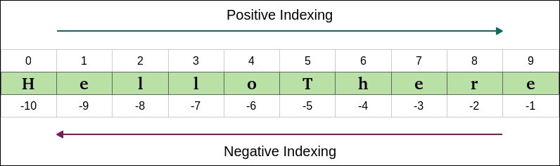
Trying to address indexes greater than 9 or smaller than -10 will raise an IndexError, as expected.
You may have noticed that, in order to keep the example as short as possible, I have called many objects using simple letters, like a, b, c, d, and so on. This is perfectly ok when you debug on the console or when you show that a + b == 7, but it's bad practice when it comes to professional coding (or any type of coding, for all that matter). I hope you will indulge me if I sometimes do it, the reason is to present the code in a more compact way.
In a real environment though, when you choose names for your data, you should choose them carefully and they should reflect what the data is about. So, if you have a collection of Customer objects, customers is a perfectly good name for it. Would customers_list, customers_tuple, or customers_collection work as well? Think about it for a second. Is it good to tie the name of the collection to the data type? I don't think so, at least in most cases. So I'd say if you have an excellent reason to do so go ahead, otherwise don't. The reason is, once that customers_tuple starts being used in different places of your code, and you realize you actually want to use a list instead of a tuple, you're up for some fun refactoring (also known as wasted time). Names for data should be nouns, and names for functions should be verbs. Names should be as expressive as possible. Python is actually a very good example when it comes to names. Most of the time you can just guess what a function is called if you know what it does. Crazy, huh?
Chapter 2, Meaningful Names of Clean Code, Robert C. Martin, Prentice Hall is entirely dedicated to names. It's an amazing book that helped me improve my coding style in many different ways, a must read if you want to take your coding to the next level.
Small values caching
When we discussed objects at the beginning of this chapter, we saw that when we assigned a name to an object, Python creates the object, sets its value, and then points the name to it. We can assign different names to the same value and we expect different objects to be created, like this:
>>> a = 1000000 >>> b = 1000000 >>> id(a) == id(b) False
In the preceding example, a and b are assigned to two int objects, which have the same value but they are not the same object, as you can see, their id is not the same. So let's do it again:
>>> a = 5 >>> b = 5 >>> id(a) == id(b) True
Oh oh! Is Python broken? Why are the two objects the same now? We didn't do a = b = 5, we set them up separately. Well, the answer is performances. Python caches short strings and small numbers, to avoid having many copies of them clogging up the system memory. Everything is handled properly under the hood so you don't need to worry a bit, but make sure that you remember this behavior should your code ever need to fiddle with IDs.
As we've seen, Python provides you with several built-in data types and sometimes, if you're not that experienced, choosing the one that serves you best can be tricky, especially when it comes to collections. For example, say you have many dictionaries to store, each of which represents a customer. Within each customer dictionary there's an 'id': 'code' unique identification code. In what kind of collection would you place them? Well, unless I know more about these customers, it's very hard to answer. What kind of access will I need? What sort of operations will I have to perform on each of them, and how many times? Will the collection change over time? Will I need to modify the customer dictionaries in any way? What is going to be the most frequent operation I will have to perform on the collection?
If you can answer the preceding questions, then you will know what to choose. If the collection never shrinks or grows (in other words, it won't need to add/delete any customer object after creation) or shuffles, then tuples are a possible choice. Otherwise lists are a good candidate. Every customer dictionary has a unique identifier though, so even a dictionary could work. Let me draft these options for you:
# example customer objects
customer1 = {'id': 'abc123', 'full_name': 'Master Yoda'}
customer2 = {'id': 'def456', 'full_name': 'Obi-Wan Kenobi'}
customer3 = {'id': 'ghi789', 'full_name': 'Anakin Skywalker'}
# collect them in a tuple
customers = (customer1, customer2, customer3)
# or collect them in a list
customers = [customer1, customer2, customer3]
# or maybe within a dictionary, they have a unique id after all
customers = {
'abc123': customer1,
'def456': customer2,
'ghi789': customer3,
}Some customers we have there, right? I probably wouldn't go with the tuple option, unless I wanted to highlight that the collection is not going to change. I'd say usually a list is better, it allows for more flexibility.
Another factor to keep in mind is that tuples and lists are ordered collections, while if you use a dictionary or a set you lose the ordering, so you need to know if ordering is important in your application.
What about performances? For example in a list, operations such as insertion and membership can take O(n), while they are O(1) for a dictionary. It's not always possible to use dictionaries though, if we don't have the guarantee that we can uniquely identify each item of the collection by means of one of its properties, and that the property in question is hashable (so it can be a key in dict).
Note
If you're wondering what O(n) and O(1) mean, please Google "big O notation" and get a gist of it from anywhere. In this context, let's just say that if performing an operation Op on a data structure takes O(f(n)), it would mean that Op takes at most a time to complete, where c is some positive constant, n is the size of the input, and f is some function. So, think of O(...) as an upper bound for the running time of an operation (it can be used also to size other measurable quantities, of course).
Another way of understanding if you have chosen the right data structure is by looking at the code you have to write in order to manipulate it. If everything comes easily and flows naturally, then you probably have chosen correctly, but if you find yourself thinking your code is getting unnecessarily complicated, then you probably should try and decide whether you need to reconsider your choices. It's quite hard to give advice without a practical case though, so when you choose a data structure for your data, try to keep ease of use and performance in mind and give precedence to what matters most in the context you are.
At the beginning of this chapter, we saw slicing applied on strings. Slicing in general applies to a sequence, so tuples, lists, strings, etc. With lists, slicing can also be used for assignment. I've almost never seen this used in professional code, but still, you know you can. Could you slice dictionaries or sets? I hear you scream "Of course not! They are not ordered!". Excellent, I see we're on the same page here, so let's talk about indexing.
There is one characteristic about Python indexing I haven't mentioned before. I'll show you by example. How do you address the last element of a collection? Let's see:
>>> a = list(range(10)) # `a` has 10 elements. Last one is 9. >>> a [0, 1, 2, 3, 4, 5, 6, 7, 8, 9] >>> len(a) # its length is 10 elements 10 >>> a[len(a) - 1] # position of last one is len(a) - 1 9 >>> a[-1] # but we don't need len(a)! Python rocks! 9 >>> a[-2] # equivalent to len(a) - 2 8 >>> a[-3] # equivalent to len(a) - 3 7
If the list a has 10 elements, because of the 0-index positioning system of Python, the first one is at position 0 and the last one is at position 9. In the preceding example, the elements are conveniently placed in a position equal to their value: 0 is at position 0, 1 at position 1, and so on.
So, in order to fetch the last element, we need to know the length of the whole list (or tuple, or string, and so on) and then subtract 1. Hence: len(a) – 1. This is so common an operation that Python provides you with a way to retrieve elements using negative indexing. This proves very useful when you do some serious data manipulation. Here's a nice diagram about how indexing works on the string "HelloThere":
Trying to address indexes greater than 9 or smaller than -10 will raise an IndexError, as expected.
You may have noticed that, in order to keep the example as short as possible, I have called many objects using simple letters, like a, b, c, d, and so on. This is perfectly ok when you debug on the console or when you show that a + b == 7, but it's bad practice when it comes to professional coding (or any type of coding, for all that matter). I hope you will indulge me if I sometimes do it, the reason is to present the code in a more compact way.
In a real environment though, when you choose names for your data, you should choose them carefully and they should reflect what the data is about. So, if you have a collection of Customer objects, customers is a perfectly good name for it. Would customers_list, customers_tuple, or customers_collection work as well? Think about it for a second. Is it good to tie the name of the collection to the data type? I don't think so, at least in most cases. So I'd say if you have an excellent reason to do so go ahead, otherwise don't. The reason is, once that customers_tuple starts being used in different places of your code, and you realize you actually want to use a list instead of a tuple, you're up for some fun refactoring (also known as wasted time). Names for data should be nouns, and names for functions should be verbs. Names should be as expressive as possible. Python is actually a very good example when it comes to names. Most of the time you can just guess what a function is called if you know what it does. Crazy, huh?
Chapter 2, Meaningful Names of Clean Code, Robert C. Martin, Prentice Hall is entirely dedicated to names. It's an amazing book that helped me improve my coding style in many different ways, a must read if you want to take your coding to the next level.
How to choose data structures
As we've seen, Python provides you with several built-in data types and sometimes, if you're not that experienced, choosing the one that serves you best can be tricky, especially when it comes to collections. For example, say you have many dictionaries to store, each of which represents a customer. Within each customer dictionary there's an 'id': 'code' unique identification code. In what kind of collection would you place them? Well, unless I know more about these customers, it's very hard to answer. What kind of access will I need? What sort of operations will I have to perform on each of them, and how many times? Will the collection change over time? Will I need to modify the customer dictionaries in any way? What is going to be the most frequent operation I will have to perform on the collection?
If you can answer the preceding questions, then you will know what to choose. If the collection never shrinks or grows (in other words, it won't need to add/delete any customer object after creation) or shuffles, then tuples are a possible choice. Otherwise lists are a good candidate. Every customer dictionary has a unique identifier though, so even a dictionary could work. Let me draft these options for you:
# example customer objects
customer1 = {'id': 'abc123', 'full_name': 'Master Yoda'}
customer2 = {'id': 'def456', 'full_name': 'Obi-Wan Kenobi'}
customer3 = {'id': 'ghi789', 'full_name': 'Anakin Skywalker'}
# collect them in a tuple
customers = (customer1, customer2, customer3)
# or collect them in a list
customers = [customer1, customer2, customer3]
# or maybe within a dictionary, they have a unique id after all
customers = {
'abc123': customer1,
'def456': customer2,
'ghi789': customer3,
}Some customers we have there, right? I probably wouldn't go with the tuple option, unless I wanted to highlight that the collection is not going to change. I'd say usually a list is better, it allows for more flexibility.
Another factor to keep in mind is that tuples and lists are ordered collections, while if you use a dictionary or a set you lose the ordering, so you need to know if ordering is important in your application.
What about performances? For example in a list, operations such as insertion and membership can take O(n), while they are O(1) for a dictionary. It's not always possible to use dictionaries though, if we don't have the guarantee that we can uniquely identify each item of the collection by means of one of its properties, and that the property in question is hashable (so it can be a key in dict).
Note
If you're wondering what O(n) and O(1) mean, please Google "big O notation" and get a gist of it from anywhere. In this context, let's just say that if performing an operation Op on a data structure takes O(f(n)), it would mean that Op takes at most a time to complete, where c is some positive constant, n is the size of the input, and f is some function. So, think of O(...) as an upper bound for the running time of an operation (it can be used also to size other measurable quantities, of course).
Another way of understanding if you have chosen the right data structure is by looking at the code you have to write in order to manipulate it. If everything comes easily and flows naturally, then you probably have chosen correctly, but if you find yourself thinking your code is getting unnecessarily complicated, then you probably should try and decide whether you need to reconsider your choices. It's quite hard to give advice without a practical case though, so when you choose a data structure for your data, try to keep ease of use and performance in mind and give precedence to what matters most in the context you are.
At the beginning of this chapter, we saw slicing applied on strings. Slicing in general applies to a sequence, so tuples, lists, strings, etc. With lists, slicing can also be used for assignment. I've almost never seen this used in professional code, but still, you know you can. Could you slice dictionaries or sets? I hear you scream "Of course not! They are not ordered!". Excellent, I see we're on the same page here, so let's talk about indexing.
There is one characteristic about Python indexing I haven't mentioned before. I'll show you by example. How do you address the last element of a collection? Let's see:
>>> a = list(range(10)) # `a` has 10 elements. Last one is 9. >>> a [0, 1, 2, 3, 4, 5, 6, 7, 8, 9] >>> len(a) # its length is 10 elements 10 >>> a[len(a) - 1] # position of last one is len(a) - 1 9 >>> a[-1] # but we don't need len(a)! Python rocks! 9 >>> a[-2] # equivalent to len(a) - 2 8 >>> a[-3] # equivalent to len(a) - 3 7
If the list a has 10 elements, because of the 0-index positioning system of Python, the first one is at position 0 and the last one is at position 9. In the preceding example, the elements are conveniently placed in a position equal to their value: 0 is at position 0, 1 at position 1, and so on.
So, in order to fetch the last element, we need to know the length of the whole list (or tuple, or string, and so on) and then subtract 1. Hence: len(a) – 1. This is so common an operation that Python provides you with a way to retrieve elements using negative indexing. This proves very useful when you do some serious data manipulation. Here's a nice diagram about how indexing works on the string "HelloThere":
Trying to address indexes greater than 9 or smaller than -10 will raise an IndexError, as expected.
You may have noticed that, in order to keep the example as short as possible, I have called many objects using simple letters, like a, b, c, d, and so on. This is perfectly ok when you debug on the console or when you show that a + b == 7, but it's bad practice when it comes to professional coding (or any type of coding, for all that matter). I hope you will indulge me if I sometimes do it, the reason is to present the code in a more compact way.
In a real environment though, when you choose names for your data, you should choose them carefully and they should reflect what the data is about. So, if you have a collection of Customer objects, customers is a perfectly good name for it. Would customers_list, customers_tuple, or customers_collection work as well? Think about it for a second. Is it good to tie the name of the collection to the data type? I don't think so, at least in most cases. So I'd say if you have an excellent reason to do so go ahead, otherwise don't. The reason is, once that customers_tuple starts being used in different places of your code, and you realize you actually want to use a list instead of a tuple, you're up for some fun refactoring (also known as wasted time). Names for data should be nouns, and names for functions should be verbs. Names should be as expressive as possible. Python is actually a very good example when it comes to names. Most of the time you can just guess what a function is called if you know what it does. Crazy, huh?
Chapter 2, Meaningful Names of Clean Code, Robert C. Martin, Prentice Hall is entirely dedicated to names. It's an amazing book that helped me improve my coding style in many different ways, a must read if you want to take your coding to the next level.
About indexing and slicing
At the beginning of this chapter, we saw slicing applied on strings. Slicing in general applies to a sequence, so tuples, lists, strings, etc. With lists, slicing can also be used for assignment. I've almost never seen this used in professional code, but still, you know you can. Could you slice dictionaries or sets? I hear you scream "Of course not! They are not ordered!". Excellent, I see we're on the same page here, so let's talk about indexing.
There is one characteristic about Python indexing I haven't mentioned before. I'll show you by example. How do you address the last element of a collection? Let's see:
>>> a = list(range(10)) # `a` has 10 elements. Last one is 9. >>> a [0, 1, 2, 3, 4, 5, 6, 7, 8, 9] >>> len(a) # its length is 10 elements 10 >>> a[len(a) - 1] # position of last one is len(a) - 1 9 >>> a[-1] # but we don't need len(a)! Python rocks! 9 >>> a[-2] # equivalent to len(a) - 2 8 >>> a[-3] # equivalent to len(a) - 3 7
If the list a has 10 elements, because of the 0-index positioning system of Python, the first one is at position 0 and the last one is at position 9. In the preceding example, the elements are conveniently placed in a position equal to their value: 0 is at position 0, 1 at position 1, and so on.
So, in order to fetch the last element, we need to know the length of the whole list (or tuple, or string, and so on) and then subtract 1. Hence: len(a) – 1. This is so common an operation that Python provides you with a way to retrieve elements using negative indexing. This proves very useful when you do some serious data manipulation. Here's a nice diagram about how indexing works on the string "HelloThere":
Trying to address indexes greater than 9 or smaller than -10 will raise an IndexError, as expected.
You may have noticed that, in order to keep the example as short as possible, I have called many objects using simple letters, like a, b, c, d, and so on. This is perfectly ok when you debug on the console or when you show that a + b == 7, but it's bad practice when it comes to professional coding (or any type of coding, for all that matter). I hope you will indulge me if I sometimes do it, the reason is to present the code in a more compact way.
In a real environment though, when you choose names for your data, you should choose them carefully and they should reflect what the data is about. So, if you have a collection of Customer objects, customers is a perfectly good name for it. Would customers_list, customers_tuple, or customers_collection work as well? Think about it for a second. Is it good to tie the name of the collection to the data type? I don't think so, at least in most cases. So I'd say if you have an excellent reason to do so go ahead, otherwise don't. The reason is, once that customers_tuple starts being used in different places of your code, and you realize you actually want to use a list instead of a tuple, you're up for some fun refactoring (also known as wasted time). Names for data should be nouns, and names for functions should be verbs. Names should be as expressive as possible. Python is actually a very good example when it comes to names. Most of the time you can just guess what a function is called if you know what it does. Crazy, huh?
Chapter 2, Meaningful Names of Clean Code, Robert C. Martin, Prentice Hall is entirely dedicated to names. It's an amazing book that helped me improve my coding style in many different ways, a must read if you want to take your coding to the next level.
About the names
You may have noticed that, in order to keep the example as short as possible, I have called many objects using simple letters, like a, b, c, d, and so on. This is perfectly ok when you debug on the console or when you show that a + b == 7, but it's bad practice when it comes to professional coding (or any type of coding, for all that matter). I hope you will indulge me if I sometimes do it, the reason is to present the code in a more compact way.
In a real environment though, when you choose names for your data, you should choose them carefully and they should reflect what the data is about. So, if you have a collection of Customer objects, customers is a perfectly good name for it. Would customers_list, customers_tuple, or customers_collection work as well? Think about it for a second. Is it good to tie the name of the collection to the data type? I don't think so, at least in most cases. So I'd say if you have an excellent reason to do so go ahead, otherwise don't. The reason is, once that customers_tuple starts being used in different places of your code, and you realize you actually want to use a list instead of a tuple, you're up for some fun refactoring (also known as wasted time). Names for data should be nouns, and names for functions should be verbs. Names should be as expressive as possible. Python is actually a very good example when it comes to names. Most of the time you can just guess what a function is called if you know what it does. Crazy, huh?
Chapter 2, Meaningful Names of Clean Code, Robert C. Martin, Prentice Hall is entirely dedicated to names. It's an amazing book that helped me improve my coding style in many different ways, a must read if you want to take your coding to the next level.
In this chapter, we've explored the built-in data types of Python. We've seen how many they are and how much can be achieved by just using them in different combinations.
We've seen number types, sequences, sets, mappings, collections, we've seen that everything is an object, we've learned the difference between mutable and immutable, and we've also learned about slicing and indexing (and, proudly, negative indexing as well).
We've presented simple examples, but there's much more that you can learn about this subject, so stick your nose into the official documentation and explore.
Most of all, I encourage you to try out all the exercises by yourself, get your fingers using that code, build some muscle memory, and experiment, experiment, experiment. Learn what happens when you divide by zero, when you combine different number types into a single expression, when you manage strings. Play with all data types. Exercise them, break them, discover all their methods, enjoy them and learn them well, damn well.
If your foundation is not rock solid, how good can your code be? And data is the foundation for everything. Data shapes what dances around it.
The more you progress with the book, the more it's likely that you will find some discrepancies or maybe a small typo here and there in my code (or yours). You will get an error message, something will break. That's wonderful! When you code, things break all the time, you debug and fix all the time, so consider errors as useful exercises to learn something new about the language you're using, and not as failures or problems. Errors will keep coming up until your very last line of code, that's for sure, so you may as well start making your peace with them now.
The next chapter is about iterating and making decisions. We'll see how to actually put those collections in use, and take decisions based on the data we're presented with. We'll start to go a little faster now that your knowledge is building up, so make sure you're comfortable with the contents of this chapter before you move to the next one. Once more, have fun, explore, break things. It's a very good way to learn.