-
Book Overview & Buying
-
Table Of Contents

Extending and Modifying LAMMPS Writing Your Own Source Code
By :
Extending and Modifying LAMMPS Writing Your Own Source Code
By:
Overview of this book
LAMMPS is one of the most widely used tools for running simulations for research in molecular dynamics. While the tool itself is fairly easy to use, more often than not you’ll need to customize it to meet your specific simulation requirements. Extending and Modifying LAMMPS bridges this learning gap and helps you achieve this by writing custom code to add new features to LAMMPS source code. Written by ardent supporters of LAMMPS, this practical guide will enable you to extend the capabilities of LAMMPS with the help of step-by-step explanations of essential concepts, practical examples, and self-assessment questions.
This LAMMPS book provides a hands-on approach to implementing associated methodologies that will get you up and running and productive in no time. You’ll begin with a short introduction to the internal mechanisms of LAMMPS, and gradually transition to an overview of the source code along with a tutorial on modifying it. As you advance, you’ll understand the structure, syntax, and organization of LAMMPS source code, and be able to write your own source code extensions to LAMMPS that implement features beyond the ones available in standard downloadable versions.
By the end of this book, you’ll have learned how to add your own extensions and modifications to the LAMMPS source code that can implement features that suit your simulation requirements.
Table of Contents (21 chapters)
Preface

Section 1: Getting Started with LAMMPS
 Free Chapter
Chapter 1: MD Theory and Simulation Practices
Chapter 2: LAMMPS Syntax and Source Code Hierarchy
Section 2: Understanding the Source Code Structure
Chapter 3: Source Code Structure and Stages of Execution
Chapter 4: Accessing Information by Variables, Arrays, and Methods
Chapter 5: Understanding Pair Styles
Chapter 6: Understanding Computes
Chapter 7: Understanding Fixes
Chapter 8: Exploring Supporting Classes
Section 3: Modifying the Source Code
Chapter 9: Modifying Pair Potentials
Chapter 10: Modifying Force Applications
Chapter 11: Modifying Thermostats
Assessments
Other Books You May Enjoy
Appendix A: Building LAMMPS with CMake
Appendix B: Debugging Programs
Appendix C: Getting Familiar with MPI
Appendix D: Compatibility with Version 29Oct20
 of velocities in a single direction i (which can be x, y, z) of a system of particles of mass m each is given by the Gaussian function, illustrated here in Figure 1.2:
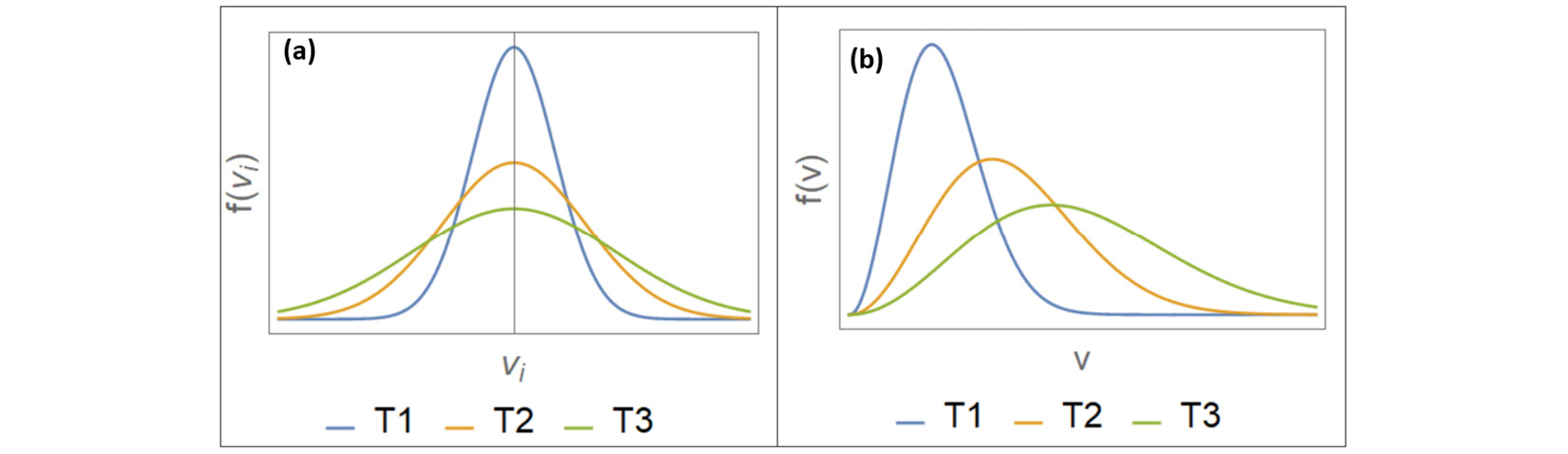
 .
.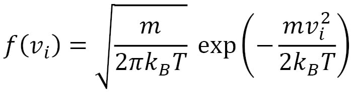
 is the Boltzmann constant. This distribution has a mean of
  and a standard deviation of
  . The shape of the Gaussian curve is determined by the ratio of
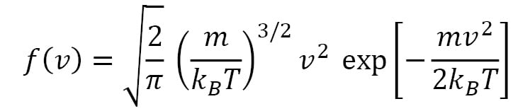
  . The velocity distribution of the velocity vector
  is given by the following formula:
 , as follows: