Book Image

Extending and Modifying LAMMPS Writing Your Own Source Code

By : Dr. Shafat Mubin, Jichen Li
Book Image

Extending and Modifying LAMMPS Writing Your Own Source Code

By: Dr. Shafat Mubin, Jichen Li

Overview of this book

LAMMPS is one of the most widely used tools for running simulations for research in molecular dynamics. While the tool itself is fairly easy to use, more often than not you’ll need to customize it to meet your specific simulation requirements. Extending and Modifying LAMMPS bridges this learning gap and helps you achieve this by writing custom code to add new features to LAMMPS source code. Written by ardent supporters of LAMMPS, this practical guide will enable you to extend the capabilities of LAMMPS with the help of step-by-step explanations of essential concepts, practical examples, and self-assessment questions. This LAMMPS book provides a hands-on approach to implementing associated methodologies that will get you up and running and productive in no time. You’ll begin with a short introduction to the internal mechanisms of LAMMPS, and gradually transition to an overview of the source code along with a tutorial on modifying it. As you advance, you’ll understand the structure, syntax, and organization of LAMMPS source code, and be able to write your own source code extensions to LAMMPS that implement features beyond the ones available in standard downloadable versions. By the end of this book, you’ll have learned how to add your own extensions and modifications to the LAMMPS source code that can implement features that suit your simulation requirements.
Table of Contents (21 chapters)
1
Section 1: Getting Started with LAMMPS
4
Section 2: Understanding the Source Code Structure
11
Section 3: Modifying the Source Code

Implementing MD simulation practices

In order to implement MD simulations that are computationally efficient and model realistic atomic systems, a number of standard simulation practices are employed. A user is likely to find these practices employed in typical Large-scale Atomic/Molecular Massively Parallel Simulator (LAMMPS) scripts and it is therefore helpful to be familiar with these concepts before delving into the LAMMPS source code. In this section, we will briefly discuss some of these practices (details are available in the MD textbooks referred to in the Introducing MD theory section).

Pair-potential cutoff

If it is desired that a potential reaches exactly zero at the cutoff, an offset () can be employed by calculating the potential at the cutoff , that is . This offset can then be subtracted from the original potential to guarantee a zero value at the cutoff, that is . Altogether, the potential with the offset changes the value of the system potential, but does not alter the forces because is a constant term that produces zero force contribution upon differentiating.

Most pair-potential functions are defined to asymptotically approach zero potential— for example, the Lennard-Jones function approaches zero as the inverse-sixth power of separation. For particles located far from each other, it implies that there exists some small but non-zero potential between them, which may be negligible in a simulation context but still adds numerical computation overhead.

Therefore, a common practice is to employ a cutoff distance for pair potentials, beyond which the interaction is assumed to be zero. The cutoff is chosen at a separation where the potential value is sufficiently small so as not to create significant errors by discounting interaction with neighbors located beyond the cutoff. During a simulation run, only the neighbors located within the cutoff radius of a particle are considered for force or potential calculations, thereby reducing computation time.

Periodic boundary conditions

Simulated systems often consist of a small cell that is representative of a larger system—for example, nanocrystal representation of a metal lattice. In such systems, it can often be assumed that the entire system is made up of many replications of the simulation box. In 1912, Born and von Karman came up with the implementation of periodic boundary conditions that can simulate a continuous replicated system starting from a simulation box.

Each wall (that is, boundary) of the simulation box is assumed to be adjacent to an identical simulation box containing identical atoms at identical positions. In effect, each wall of the box leads to a replica of the simulation box, containing images of the same atoms as in the simulation box. At every iteration, as the atom positions in the simulation box are updated, the image atoms in the replicas are accordingly updated. The following diagram shows this simulation box:

Figure 1.3 – A 2D simulation box without (top) and with (bottom) periodic boundaries

Figure 1.3 – A 2D simulation box without (top) and with (bottom) periodic boundaries

In this diagram, we see the following:

  • Top: A snapshot of a 2D simulation box consisting of four particles (indexed from 1 to 4) without periodic boundaries.
  • Bottom: The same simulation box with periodic boundaries in all directions produces 8 replicas (26 replicas in 3D) containing image atoms (dashed circles). At every iteration, all replicas are identically updated by replicating the particles in the central simulation box.

This way, enclosing wall boundaries are eliminated, and any atom that exits the simulation box by passing through a wall will automatically re-enter through the opposite wall, thus conserving the number of atoms and modeling continuous motion of atoms. Furthermore, the atoms in the simulation box are permitted to interact with the image atoms located in the replicas, ensuring that atoms located near to the walls are not considered as fringe atoms with few neighbors only because of their remoteness from the box center.

In Figure 1.3, in the absence of periodic boundaries, particle 3 at the top-right corner is observed to be located far from particles 1 and 4, and would undergo reduced or zero interactions with these particles. By contrast, when periodic boundaries are implemented, particle 3 is located considerably closer to images of particles 1 and 4.

Subsequently, particle 3 is able to interact with other particles located in all directions around itself as if it were contained in a continuous, unbounded simulation box. At the same time, consistency of interaction requires that particle 3 interacts with either an image or with the original particle in the simulation box, but not both together, and it is accomplished by setting the side lengths of the simulation box to be at least double the pair-potential cutoff distance between atoms. This requirement is known as the minimum image convention, which guarantees that pair-potential interactions are not double-counted.

Long-range electrostatic potentials decay considerably slower than many other interactions (as inverse of the separation) and would therefore require disproportionately long cutoffs and correspondingly large simulation boxes to model with a traditional pair potential. To circumvent this problem, electrostatic interactions with image atoms are summed up by an Ewald summation (or a related particle-mesh method) that divides the calculation to a real-space component and a reciprocal-space component. This way, a cutoff is not required, but periodic boundaries are necessary to ensure sum convergence.

When an atom exits a simulation box and its image enters from the opposite side of the box, the atom coordinates can extend beyond the simulation box coordinates. This is accounted for using the concept of wrapped and unwrapped coordinates, where unwrapped coordinates represent the unadjusted atom coordinates and wrapped coordinates represent the coordinates adjusted by resetting to the coordinates of the re-entry wall.

In LAMMPS, trajectory output files may include an image flag to keep track of wrapped and unwrapped coordinates. When an atom exits the simulation box along the positive direction in any dimension, the image flag corresponding to this axis would increment by one. Accordingly, the image flag decrements by one if the atom exits along the negative direction. Thus, the image flag of an atom multiplied by the corresponding simulation box side length can be used to convert from wrapped to unwrapped coordinates.

Neighbor lists

An atom only interacts with its neighbors located within a cutoff radius, and these neighbors are identified by calculating their distances from the atom in consideration. For a system of N atoms, this could lead to calculating the distance between each of the 
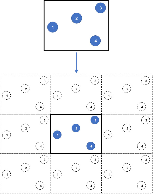
pairs of atoms. To reduce the computation overhead, for every atom a subset of neighbors is selected into a neighbor list (suggested by Verlet in 1967), and only these short-listed neighbors are used to calculate the interactions with the atom.
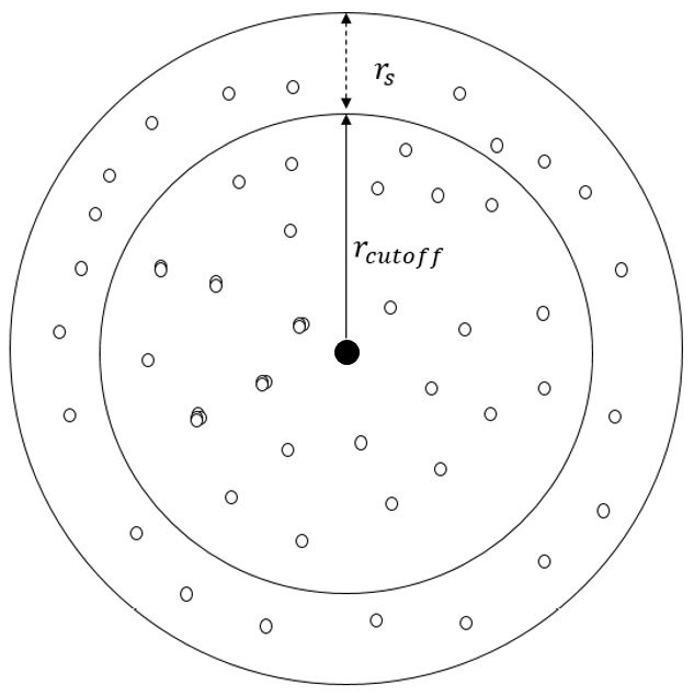
At the beginning of a simulation, a neighbor list is built for every interacting atom in the system by tagging all its neighboring atoms that lie within its cutoff or within a short buffer width, known as the skin width (shown in Figure 1.4). If the atoms are not traveling at extreme speeds, only the atoms located within the cutoff or the skin (that is, the neighbor-list members) at a certain iteration can be expected to lie inside the cutoff radius in the next iteration, and it can be expected that no atom previously located outside the skin will be able to cross inside the cutoff radius in the space of one iteration.

This way, the neighbor list excludes atoms that are located sufficiently far by reusing information from the preceding iteration, and this therefore reduces computation time in calculating neighbor distances. The process is illustrated in the following diagram:

Figure 1.4 – Illustration of the radial cutoff distance  and 
the skin width  of a central atom (black dot)

Figure 1.4 – Illustration of the radial cutoff distance and the skin width of a central atom (black dot)

At any timestep, the atoms that are located inside are included in the neighbor list of the central atom, whereas only the atoms located inside interact with the central atom. At the next iteration, only the atoms tagged in the neighbor list are considered when identifying atoms that can interact with the central atom, and the neighbor list may be rebuilt depending on the displacements of the atoms.

Generally, the neighbor lists do not have to be rebuilt at every iteration, and the interval between rebuilding can be defined by the user. Also, a common practice is to rebuild only when an atom has traveled more than half the skin width since the previous neighbor-list build. It also implies that a larger skin width requires less frequent neighbor-list builds, at the cost of including a greater number of neighbors per list at every iteration.

The skin width can be specified independently of the cutoff distance and is generally chosen according to timestep and expected particle velocities. At the lower limit, the skin width should be double the maximum displacement expected of a particle in an iteration. In LAMMPS, if an atom is able to cross the skin width in one iteration, the associated neighbor lists experience a dangerous build whereby the loss of the atom can lead to errors in force calculations and violation of energy conservation. If a dangerous build is detected, the neighbor list needs to be rebuilt to rectify this.

When a neighbor list is used to calculate the interaction force between a pair of atoms, the two atoms in the pair can be assigned equal and opposite forces by Newton's third law. This equivalency can be enabled using a full-neighbor list, whereas it can be disabled by using a half-neighbor list. While a full-neighbor list reduces computation cost, half-neighbor lists may be preferred in simulations where equal and opposite forces are not applicable.

Processor communication

Modern parallel computers have two main forms: shared-memory machines, where multiple processors (often called cores) access the same memory; and distributed-memory machines, where a processor (often called a node) cannot access the memory designated to another processor. Modern high-performance computing facilities are all based on a hybrid architecture. A node consists of multiple cores, and many nodes combine to form a supercomputer. This architecture also leads to an issue of distributing the workload and allocating tasks between nodes and cores.

In the context of MD, one strategy that addresses the task allocation problem is spatial decomposition, which divides the simulation box into equal sections and assigns atoms located in each section to a different core, as shown here:

Figure 1.5 – (Left) A single processing core calculating the trajectory of every atom 
in the simulation box. (Right) The simulation box is divided into domains, 
and the atoms in each domain are assigned to a different core

Figure 1.5 – (Left) A single processing core calculating the trajectory of every atom in the simulation box. (Right) The simulation box is divided into domains, and the atoms in each domain are assigned to a different core

The domains in the preceding diagram are spatially decomposed by volume. Copies of atoms, known as ghost atoms, are exchanged between processors to account for interactions between atoms located on different cores. Each core calculates the interactions of atoms assigned to it in parallel and thereby increases the overall simulation speed.

To account for interactions between atoms located on different cores, each core builds its domain with a shell that accommodates particles located at the edges of a domain, and exchanges copies of particles (known as ghost atoms) with other cores, as illustrated in the following diagram:

Figure 1.6 – A core domain showing its shell (dashed box) and 
ghost atoms shared with a neighboring domain

Figure 1.6 – A core domain showing its shell (dashed box) and ghost atoms shared with a neighboring domain

There are two stages of communication between cores involved, detailed here:

  • In the first stage, the shell exchanges the ghost-atom coordinates with neighboring cores to register the particles that can interact with the particles contained in the domain. The ghost atoms in these shells are essentially images of atoms in other domains.
  • In the second stage, the updated atom positions at the following iteration are used to determine whether any atom has moved to a different domain, and if so, the atom coordinates and kinematics information are communicated to the appropriate cores. After this step, the particles in the shell are deleted from the memory.

This parallel mechanism demonstrates that communication time between cores multiplies as the number of cores increases. Due to memory and bandwidth limits, parallelization cannot achieve the ideal optimization of 
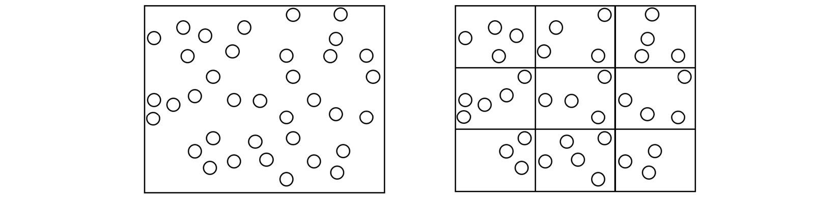
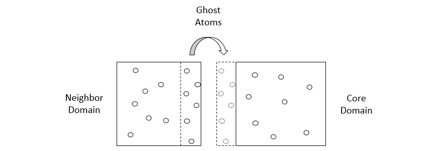
, where N is the number of atoms and P is the number of processors, and leads to a sub-linear speedup. Therefore, for a given simulation system an increasing number of cores eventually reduces efficiency, and there exists an optimum number of cores that delivers the best performance.