2.1. Postulate 1 – Wave functions

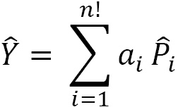
The total wave function describes the physical behavior of a system and is represented by the capital Greek letter Psi: . It contains all the information of a quantum system and includes complex numbers () as parameters. In general, is a function of all the particles in the system , where the total number of particles is . Furthermore, includes the spatial position of each particle (), the spin directional coordinates for each particle (), and time :

where and are vectors of single-particle coordinates:

The total wave function for a one-particle system is a product of a spatial , spin , and time functions:

If the wave function for a multiple-particle system cannot be factored into a product of single-particle functions, then we consider the quantum system as entangled. If the wave function can be factored into a product of single-particle functions, then it is not entangled and is called a separable state. We will revisit the concept of entanglement in Chapter 3, Quantum Circuit Model of Computation.

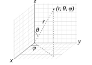
The spatial part of the wave function can be converted from Cartesian coordinates to spherical coordinates where is the radial distance determined by the distance formula , is the polar angle ranging from 0 to (), and is the azimuthal angle ranging from 0 to (), through the following equations:

• 
• 
• 

Figure 2.3 – Spherical coordinates [public domain]

There are certain properties of a wave function that need to be properly considered in order to accurately represent a quantum system:

• Single-valued, meaning that for a given input variable there is only one possible output
• Positive definite, meaning that the complex conjugate transpose of the wave function, indicated by a dagger (, times the wave function itself is strictly greater than zero:
• Square integrable, meaning that the positive definite product is less than infinity when integrated over all space (: , where
• Normalizable, meaning that a particle must exist in a volume ( and at a point in time, that is, it must exist somewhere in all space and time: , where
• Complete, meaning that all statistically important data that is needed to represent that quantum system is available such that calculations of properties converge to a limit, that is, a single value

For quantum chemistry applications, we will use Python code to show how to include the spatial and spin functions:

• Section 2.1.1, Spherical harmonic functions, which are related to the quantum numbers and to the spatial variables or
• Section 2.1.2, Addition of momenta using Clebsch-Gordan (CG) coefficients, which is for coupling multiple particles and can be applied to both orbital ( and spin quantum numbers ()
• Section 2.1.3, The general formulation of the Pauli exclusion principle, which ensures the proper symmetry requirements for a multiple particle system: either totally fermionic, totally bosonic, or a combination of the two

From a machine learning perspective, there are other parameters that the wave function can depend on. These parameters are called hyperparameters and are used to optimize the wave function to obtain the most accurate picture of the state of interest.

2.1.1. Spherical harmonic functions

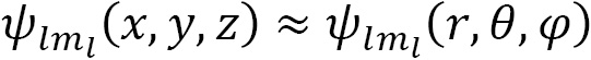
Spherical harmonic functions are used to describe one-electron systems and depend on the angular momentum () and the magnetic quantum number (), as well as the spatial coordinates:

and are a set of special functions defined on the surface of a sphere called the radial wave function :

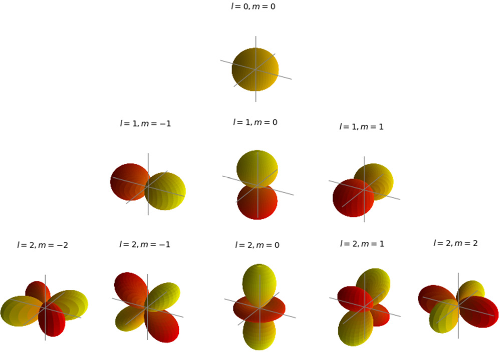
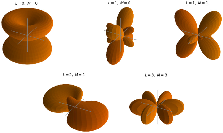
Since the hydrogen atom is the simplest atom, consisting of only one electron around a single proton, in this section we will illustrate what these functions look like. Some of the spherical harmonic functions for the hydrogen atom are shown in Figure 2.4:

Figure 2.4 – Spatial wave functions of the hydrogen atom with quantum numbers and

Recall the following:

• The principal quantum () is a continuous quantum variable that ranges from 1 to infinity such that in practice, due to ionization, it becomes a discrete variable.
• The angular momentum quantum number () is contained in the discrete set determined: .
• The magnetic quantum number () is contained in the discrete set determined by the angular momentum quantum number ():

The spherical harmonic functions, , can be split into a product of three functions:

,

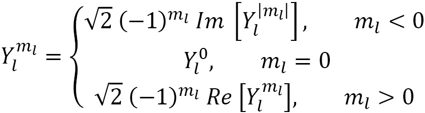
where is a constant that depends only on the quantum numbers , is a polar function, also known as the associated Legendre polynomial functions, which can be a complex function if the angular momentum () is positive or negative, and is a complex exponential azimuthal function. To illustrate spherical harmonic functions, we use the following code, which computes them [SciPy_sph], then casts them into the following real functions [Sph_Real]:

and finally displays these real functions in three dimensions with Python's Matplotlib module. Let's now implement this in Python.

Importing NumPy, SciPy, and Matplotlib Python modules

The following Python statements import the required NumPy, SciPy, and Matplotlib modules:

import numpy as np
import matplotlib.pyplot as plt
import matplotlib.gridspec as gridspec
from scipy.special import sph_harm

Setting-up grids of polar (theta ) and azimuthal (phi ) angles

We define a function called setup_grid() that creates a grid of polar coordinates and the corresponding cartesian coordinates with the following Python functions:

• numpy.linspace: Returns evenly spaced numbers over a specified interval
• numpy.meshgrid: Returns coordinate matrices from coordinate vectors

The setup_grid() function has one input parameter, num, which is a positive integer that is the number of distinct values of polar coordinates.

It returns the following:

• theta, phi: Two-dimensional NumPy arrays of shape num x num
• xyz: Three-dimensional NumPy array of shape (3,num,num)

def setup_grid(num=100):
  theta = np.linspace(0, np.pi, num)
  phi = np.linspace(0, 2*np.pi, num)
  # Create a 2D meshgrid from two 1D arrays of theta, phi coordinates
  theta, phi = np.meshgrid(theta, phi)
  # Compute cartesian coordinates with radius r = 1
  xyz = np.array([np.sin(theta) * np.sin(phi),
                np.sin(theta) * np.cos(phi),
                np.cos(theta)])
  return (theta, phi, xyz)

Let's check the shape of the NumPy arrays returned by setup_grid():

(theta, phi, xyz) = setup_grid()
print("Shape of meshgrid arrays, theta: {}, phi: {}, xyz: {}".format(theta.shape, phi.shape, xyz.shape))

Here's the output:

Shape of meshgrid arrays, theta: (100, 100), phi: (100, 100), xyz: (3, 100, 100)

Coloring the plotted surface of the real functions of the spherical harmonic function (Y)

We define a function called colour_plot() that colors the plotted surface of the real functions of the spherical harmonic according to the sign of its real part, . It has the following input parameters:

• ax: A three-dimensional Matplotlib figure
• Y: A spherical harmonic function
• Yx,Yy,Yz: Cartesian coordinates of the plotted surface of the spherical harmonic function
• cmap: A built-in colormap accessible via the matplotlib.cm.get_cmap function [Cmap], for instance, autumn, cool, spring, and winter:

def colour_plot(ax, Y, Yx, Yy, Yz, cmap):
  # Colour the plotted surface according to the sign of Y.real
  # https://matplotlib.org/stable/gallery/mplot3d/surface3d.html?highlight=surface%20plots
  # https://matplotlib.org/stable/tutorials/colors/colormaps.html
  cmap = plt.cm.ScalarMappable(cmap=plt.get_cmap(cmap))
  cmap.set_clim(-0.5, 0.5)
  ax.plot_surface(Yx, Yy, Yz,
                  facecolors=cmap.to_rgba(Y.real),
                  rstride=2, cstride=2)
  return

Defining a function that plots a set of x, y, z axes and sets the title of a figure

We define a function called draw_axes() that plots the axes of a Matplotlib figure and sets a title. It has three input parameters:

1. ax: A three-dimensional Matplotlib figure
2. ax_lim: A positive real number that controls the size of the plotted surface
3. title: A string of characters that will be shown as the title of the output figure:

def draw_axes(ax, ax_lim, title):
  ax.plot([-ax_lim, ax_lim], [0,0], [0,0], c='0.5', lw=1, zorder=10)
  ax.plot([0,0], [-ax_lim, ax_lim], [0,0], c='0.5', lw=1, zorder=10)
  ax.plot([0,0], [0,0], [-ax_lim, ax_lim], c='0.5', lw=1, zorder=10)
  # Set the limits, set the title and then turn off the axes frame
  ax.set_title(title)
  ax.set_xlim(-ax_lim, ax_lim)
  ax.set_ylim(-ax_lim, ax_lim)
  ax.set_zlim(-ax_lim, ax_lim)
  ax.axis('off')
  return

Defining a function that computes the real form of the spherical harmonic function (Y)

Please be cautious in this part of the code because SciPy defines theta () as the azimuthal angle and phi () as the polar angle [SciPy_sph], which is opposite of the standard definitions used for plotting.

The comb_Y() function takes the following input parameters:

• l: Angular momentum quantum number
• m: Magnetic quantum number
• theta, phi: Two-dimensional NumPy arrays of shape num x num

It returns the real form of the spherical harmonic function presented earlier:

def comb_Y(l, m, theta, phi):
  Y = sph_harm(abs(m), l, phi, theta)
  if m < 0:
    Y = np.sqrt(2) * (-1)**m * Y.imag
  elif m > 0:
    Y = np.sqrt(2) * (-1)**m * Y.real
  return Y

Defining a function that displays the spatial wave functions for a range of values of the angular momentum quantum number and the magnetic quantum number

The following function displays spatial wave functions for in range , where is a parameter and is in range as illustrated in the following code for the hydrogen atom in states :

def plot_orbitals(k, cmap = 'autumn'):
  for l in range(0, k+1):
    for m in range(-l, l+1):
      fig = plt.figure(figsize=plt.figaspect(1.))
      (theta, phi, xyz) = setup_grid()
      ax = fig.add_subplot(projection='3d')
      Y = comb_Y(l, m, theta, phi)
      title = r'$l={{{}}}, m={{{}}}$'.format(l, m)
      Yx, Yy, Yz = np.abs(Y) * xyz
      colour_plot(ax, Y, Yx, Yy, Yz, cmap)
      draw_axes(ax, 0.5, title)
      fig_name = 'Hydrogen_l'+str(l)+'_m'+str(m)
      plt.savefig(fig_name)
      plt.show()
  return

Spatial wave functions of the hydrogen atom

The spatial wave functions for the one electron of the hydrogen atom in states , and in range are computed and displayed with the plot_orbitals Python function defined earlier:

plot_orbitals(2)

The result is shown in Figure 2.4.

Questions to consider

What happens to the spherical harmonic functions when we have more than one electron, that is, in heavier elements? How do these functions operate or change? For instance, what happens when there are three electrons with non-zero angular momentum, as in the case with the nitrogen atom?

To accomplish this kind of complexity and variability, we need to add or couple angular momentum using Clebsch-Gordon (CG) coefficients, as presented in Section 2.1.2, Addition of momenta using CG coefficients.

2.1.2. Addition of momenta using CG coefficients

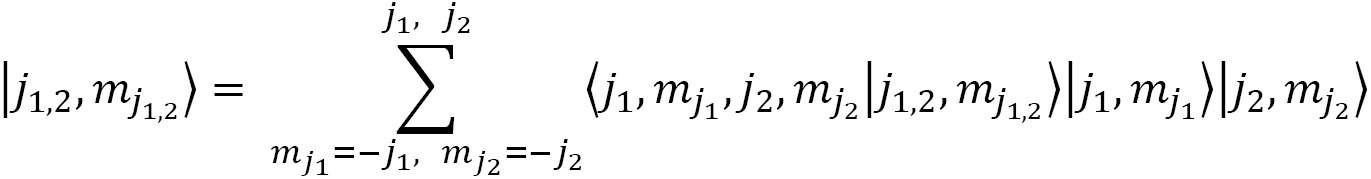
The addition or coupling of two momenta ( and ) along with the associated projections (and ) is described by the summation of two initial state wave functions and over the possible or allowed quantum numbers:

to a final state wave function of choice . Yes, we can choose the final state as we please, if we follow the rules of vector addition. The CG coefficients are the expansion coefficients of coupled total angular momentum in an uncoupled tensor product basis:

We use a generic and to represent a formula where either angular ( and ) and/or spin ( and ) momentum can be coupled together. We can couple angular momenta only, or spin momenta only, or the two together. The addition is accomplished by knowing the allowed values for the quantum numbers.

Using CG coefficients with Python SymPy

The Python SymPy library [SymPy_CG] implements the formula with the CG class as follows.

Class has the following parameters:

• : Angular momentum and the projection of state 1
• : Angular momentum the projection of state 2
• : Total angular momentum of the coupled system

Importing the SymPy CG coefficients module

The following statements import the SymPy CG coefficients module:

import sympy
from sympy import S
from sympy.physics.quantum.cg import CG, cg_simp

Defining a CG coefficient and evaluating its value

We can couple two electrons (fermions) in a spin paired state in two different ways: symmetric or antisymmetric. We denote spin up in the direction as and spin down in the direction as .

We can also couple spin states with angular momentum states. When coupling angular momentum () with spin (), we change the notation to . We go through these three examples next.

Fermionic spin pairing to symmetric state ()

The coupling of the symmetric spin paired state is and is described by the following equation:

=

Using the following code, we obtain the CG coefficients for the preceding equation:

CG(S(1)/2, S(1)/2, S(1)/2, -S(1)/2, 1, 0).doit()
CG(S(1)/2, -S(1)/2, S(1)/2, S(1)/2, 1, 0).doit()

Here's the result:

Figure 2.5 – Defining a CG coefficient and evaluating its value

Plugging in the CG coefficients as well as the up-spin and down-spin functions, we get this:

Fermionic spin pairing to antisymmetric state ()

The coupling of the antisymmetric spin paired state, , is described by the following equation:

=

Using the following code, we obtain the CG coefficients for the preceding equation:

CG(S(1)/2, S(1)/2, S(1)/2, -S(1)/2, 0, 0).doit()
CG(S(1)/2, -S(1)/2, S(1)/2, S(1)/2, 0, 0).doit()

Here's the result:

Figure 2.6 – Defining a CG coefficient and evaluating its value

Plugging in the CG coefficients as well as the up-spin and down-spin functions, we get the following:

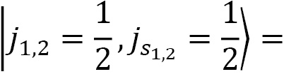
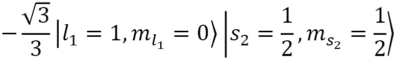
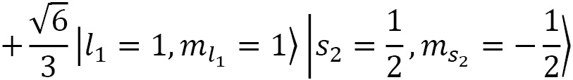
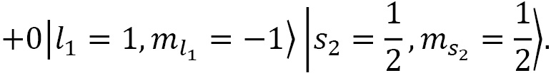
Coupling spin and angular momentum ()

Let's couple together angular momenta with and to a fermionic spin state and for a final state of choice of :

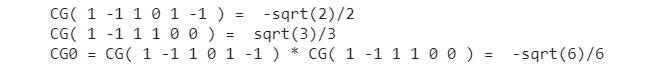
The CG coefficients of this equation are calculated using the following code:

CG(1, 0, S(1)/2, S(1)/2, S(1)/2, S(1)/2).doit()
CG(1, 1, S(1)/2, -S(1)/2, S(1)/2, S(1)/2).doit()
CG(1, -1, S(1)/2, S(1)/2, S(1)/2, S(1)/2).doit()

Here's the result:

Figure 2.7 – Defining a CG coefficient and evaluating its value

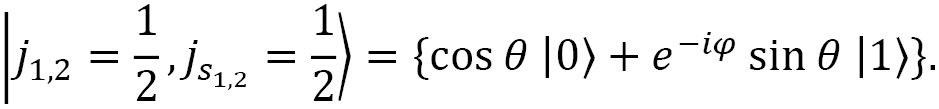
Plugging the result of the preceding code into the formula, we obtain the following:

Now, we reduce this and plug in the up-spin and down-spin functions:

In the last step, we plugged in the spherical harmonic functions for the following:

• 
• 

In doing so, we obtain this:

Then we can drop the factor of , as it is a global factor, so that the final state is as follows:

Some of you might recognize this function as a qubit wave function for computing without including time dependence. In fact, for the state of a qubit, we change the up arrow () to ket 0 () to indicate the magnetic projection of zero (), and likewise for the down arrow () to ket 1 () to indicate the magnetic projection of zero (). With this, we have the following:

We cover this topic in more detail in Chapter 3, Quantum Circuit Model of Computation.

Spatial wave functions of different states of the nitrogen atom with three p electrons

Now we would like to illustrate the wave function of the nitrogen atom with three electrons [Sharkey_0]. We chose this system because we are coupling more than two non-zero momentum vectors by expressing its coupled total momentum in an uncoupled tensor product basis of each electron [Phys5250]. This means that we assumed the wave function is not entangled. We must apply the addition of angular momenta formula twice (recursively) so that we have all the combinations of coupling with the final state of choice. The different shapes of the spatial wave function of the nitrogen atom with three electrons are shown here:

Figure 2.8 – Spatial wave functions of different states of the nitrogen atom with three electrons

We will go through the example for the final state of, .

Spatial wave function of the ground state of the nitrogen atom with 3 electrons in ,

Electrons are fermions, and therefore they cannot occupy the same set of quantum numbers. Because we are working with three electrons, the orbital angular momentum () for each electron is as follows:

and .

This couples with the final momentum state of The allowable set of magnetic momenta () for each electron is as follows:

and ,

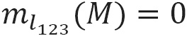
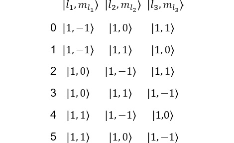
and the final coupled magnetic projection state is:

To accomplish this type of coupling of three momenta, we must apply the addition of angular momenta formula twice (recursively) so that we have all the combinations of coupling with the final state, .

Each electron is in the same shell or principal quantum number () level; however, each is in a different subshell ( and has a spin of either up or down. For this example, the spin state is irrelevant, and we are choosing to not include it. Since these electrons are in different subshells, that means they cannot have the same combination of quantum numbers ( and ):

Figure 2.9 – Electron configurations of ,

Setting up a dictionary of six configuration tuples

Each tuple contains , where is the first coupling from electron 1 with 2, and is the second coupling of electrons 1 and 2 with 3:

T00 = {0: (1,-1, 1,0,  1,-1, 1,1,  0,0), 
       1: (1,-1, 1,1,  1,0,  1,0,  0,0),
       2: (1,0,  1,-1, 1,-1, 1,1,  0,0),
       3: (1,0,  1,1,  1,1,  1,-1, 0,0),
       4: (1,1,  1,-1, 1,0,  1,0,  0,0),
       5: (1,1,  1,0,  1,1,  1,-1, 0,0)}

Defining a function that computes a product of CG coefficients

The comp_CG() function has the following input parameters:

• : Dictionary of configuration tuples
• : Index of the array in the dictionary
• : None by default, set to True to display the computation

It returns the following product of CG coefficients pertaining to the entry :

• 

def comp_CG(T, k, display = None):
  CGk = CG(*T[k][0:6]) * CG(*T[k][4:10])
  if display:
    print('CG(', *T[k][0:6], ') = ', CG(*T[k][0:6]).doit())
    print('CG(', *T[k][4:10], ') = ', CG(*T[k][4:10]).doit())
    print("CG{} =".format(k), 'CG(', *T[k][0:6], ') * CG(', *T[k][4:10], ') = ', CGk.doit())
  return CGk

For instance, for and with the display option set to True, use the following:

CG0 = comp_CG(T00, 0, display=True)

We get the following detailed output:

Figure 2.10 – Output of comp_CG for the first entry in the T00 dictionary

Computing and printing the CG coefficients

The following Python code calls the comp_CG() function for each entry in the T00 dictionary and prints the result of the computation of the CG coefficients:

for k in range(0, len(T00)):
  s = 'CG' + str(k) +' = comp_CG(T00, ' + str(k) + ')'
  exec(s)
s00 = ["CG0: {}, CG1: {}, CG2: {}, CG3: {}, CG4: {}, CG5: {}".
     format(CG0.doit(), CG1.doit(), CG2.doit(), CG3.doit(), CG4.doit(), CG5.doit())]
print(s00)

Here's the result:

Figure 2.11 – CG coefficients for computing the ground state of the nitrogen atom with three electrons (, )

Defining a set of spatial wave functions

Since electrons in the same orbital repel one another, we define a set of spatial wave functions, adding a phase of and in the wave functions of the second and third electron respectively:

def Y_phase(theta, phi):
  Y10a = comb_Y(1, 0, theta, phi)
  Y11a = comb_Y(1, 1, theta, phi)
  Y1m1a = comb_Y(1, -1, theta, phi)
  Y10b = comb_Y(1, 0, theta, phi+1*np.pi/3)
  Y11b = comb_Y(1, 1, theta, phi+1*np.pi/3)
  Y1m1b = comb_Y(1, -1, theta, phi+1*np.pi/3)
  Y10c = comb_Y(1, 0, theta, phi+2*np.pi/3)
  Y11c = comb_Y(1, 1, theta, phi+2*np.pi/3)
  Y1m1c = comb_Y(1, -1, theta, phi+2*np.pi/3)
  return(Y10a, Y11a, Y1m1a, Y10b, Y11b, Y1m1b, Y10c, Y11c, Y1m1c)

Computing the wave function of the Nitrogen atom with three electrons (, )

We compute the wave function as a sum of the products of the wave functions defined previously:

def compute_00_Y(ax_lim, cmap, title,  fig_name):
  fig = plt.figure(figsize=plt.figaspect(1.))
  (theta, phi, xyz) = setup_grid()
  ax = fig.add_subplot(projection='3d')
  (Y10a, Y11a, Y1m1a, Y10b, Y11b, Y1m1b, Y10c, Y11c, Y1m1c) = Y_phase(theta, phi)
  Y_00 = float(CG0.doit()) * Y1m1a * Y10b * Y11c
  Y_01 = float(CG1.doit()) * Y1m1a * Y11b * Y10c
  Y_02 = float(CG2.doit()) * Y10a * Y1m1b * Y11c
  Y_03 = float(CG3.doit()) * Y10a * Y11b * Y1m1c
  Y_04 = float(CG4.doit()) * Y11a * Y1m1b * Y10c
  Y_05 = float(CG5.doit()) * Y11a * Y10b * Y1m1c
  Y = Y_00 + Y_01 + Y_02 + Y_03 + Y_04 + Y_05
  Yx, Yy, Yz = np.abs(Y) * xyz
  colour_plot(ax, Y, Yx, Yy, Yz, cmap)
  draw_axes(ax, ax_lim, title)
  plt.savefig(fig_name)
  plt.show()
  return

Displaying the wave function of the ground state of the nitrogen atom with three electrons (, )

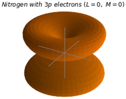
We now show the graphical representation of the spherical harmonic function for the ground state of the nitrogen atom with three electrons:

title = '$Nitrogen\ with\ 3p\ electrons\ (L=0,\ M=0)$'
fig_name ='Nitrogen_3p_L0_M0.png'
compute_00_Y(0.01, 'autumn', title, fig_name)

Here's the result:

Figure 2.12 – Spatial wave function of the ground state of the nitrogen atom with three electrons

(, )

2.1.3. General formulation of the Pauli exclusion principle

Remember that fermions are particles that have half-integer spin () and bosons are particles that have integer spin (). The general formulation of the PEP states the total wave function for a quantum system must have certain symmetries for all sets of identical particles, that is, electrons and identical nuclei, both boson and fermions, under the operation of pair particle permutation [Bubin]:

• For fermions, the total wave function must be antisymmetric () with respect to the exchange of identical pair particles :

meaning that the spatial part of the wave function is antisymmetric while the spin part is symmetric, or vice versa.

• For bosons, the total wave function must be symmetric () with respect to the exchange of pair particles ():

meaning that both the spatial wave function and spin function are symmetric, or both are antisymmetric.

• For composite systems with both identical fermions and identical bosons, the preceding operations must hold true simultaneously.

In general, the symmetrizer and antisymmetrizer operations combined for a given quantum system are referred to as the projection operator . The total wave function (, including the PEP, is then written as:

For a given quantum system, the projection operator that satisfies the PEP is obtained as a product of the antisymmetrizer and the symmetrizer, , and strictly in this order, not . Making this mistake in a calculation will result in incorrect operations.

The projection operator can be expressed as a linear combination:

where the index indicates a particular order of particles in a set of possible orders, is the permutation associated with a particular order, an associated expansion coefficient, and is the total number of identical particles. This equation is dependent on a factorial () relation of permutations, making this a non-deterministic polynomial time hard (NP-hard) computation. Please note that you cannot add and subtract operations, you can only combine like terms. As the system grows larger in the number of identical particles, the complexity increases exponentially, making this an NP-hard calculation.

The process of determining the symmetrizer and antisymmetrizer for the projection operation to apply PEP to a given quantum system is as follows:

• Identify all sets of identical particles , that is, electrons and nuclei, and fermions and bosons. Please do not confuse this for the identical number of particles with the principal quantum number as we are using the same notation.
• Build a partition function for positive integers. Remember we only have a positive count of particles, not a negative count. A partition of a positive integer is a sequence of positive integers such that and , where is the last possible integer for the set.
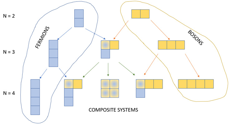
• Then use the partition to build a Young frame. A Young frame (diagram) is a series of connected boxes organized in rows that are left-aligned and arranged so that every row contains an equal or lower number of boxes than the row above it.

The totally symmetric irreducible representation of a system with identical bosons is a vertical Young tableau of boxes. The totally antisymmetric irreducible representation of a system with identical fermions and total quantum spin , is a horizontal Young tableau of boxes. We calculate the symmetry quantum () number as:

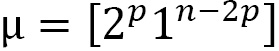
The partition function describes how to build a Young frame. There are two boxes in the first rows and one box in the remaining rows, which we write as follows:

Please note that the superscripts are not exponents. The convention for filling the numbers in the boxes is increasing from left to right, and second increasing from top to bottom. Here are some examples of how to put together the Young frame:

• When there are two identical boson particles () with total spin , the symmetry quantum number is , the partition function is , and the corresponding Young frames is:

Figure 2.13 – Young frame for the partition function

This Young frame corresponds to a totally symmetric operation.

• When there are two identical boson particles with total spin , the symmetry quantum number is , the partition function is , and the corresponding Young frame is the same as the previous Young frame.
• When there are two identical fermion particles with total spin , the symmetry quantum number is , the partition function is , and the corresponding Young frame is the same as the previous Young frame. We use this state in Section 2.2.2, Probability amplitude for a hydrogen anion .
• When there are two identical fermion particles with total spin , the symmetry quantum number is , the partition function is , and the corresponding Young frame is as follows:

Figure 2.14 – Young frame for the partition function

This Young frame corresponds to a totally antisymmetric operation.

• When there are three identical fermion particles (), with the total spin , that is, two paired electrons and one lone electron, the symmetry quantum number is , the partition function is , and the corresponding Young frame is as follows:

Figure 2.15 – Young frame for the partition function

This Young frame corresponds to both symmetric and antisymmetric operations combined.

• When there are three identical fermion particles (), with the total spin , that is, three unpaired electrons, the symmetry quantum number is , the partition function is , and the corresponding Young frame is as follows:

Figure 2.16 – Young frame for the partition function

• For the four electrons in lithium hydride (LiH), with spin pairing (), the symmetry quantum number , the partition is , and we have the following Young frame:

Figure 2.17 – Young frame for the partition function

In this example, since the nucleus is the only particle of its kind, we do not include it in the numbering of the set.

We can generalize the Young frame for fermions, bosons, and composite systems as shown in Figure 2.18.

Figure 2.18 – Young frames for fermions, bosons, and composite systems [authors]

The frame() function creates a Young frame given a partition as input:

• mu: This partition is represented as a dictionary whose keys are the partition integers and the values are the multiplicity of that integer. For example, is represented as {2: 1, 1:0}.

It returns a Young frame as follows:

• f: A dictionary of lists whose keys are the index of the lines starting from 0 and the values are the list of integers in the corresponding line. For example, represents the Young frame Figure 2.15 where the first line contains 1,2 and the second line 3:

def frame(mu):
  a = 0
  b = 0
  f = {}
  for k, v in mu.items():
    for c in range(v):
      f[a] = list(range(b+1, b+k+1))
      a += 1
      b += k
  return f

Let's run the frame() function with :

print("F_21_10 =", frame({2: 1, 1:0}))

Here is the result:

Let's run the frame() function with :

print("F_21_11 =", frame{2: 1, 1:1}))

Here is the result:

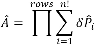
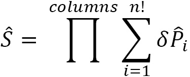
Now we are ready to define the antisymmetrizer () and symmetrizer () operations for many particles in the system that are governed by the Young frame we determined. The antisymmetrizer operator () for the rows of the Young frame is:

where is positive for odd permutations and negative for even permutations. An odd permutation has an antisymmetric permutation matrix. An even permutation has a symmetric permutation matrix. We also define a symmetrizer operator () for the columns of the Young frame:

Recall that the projection operator is then the product: .

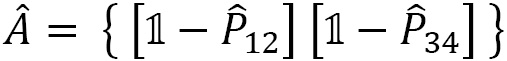
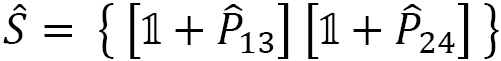
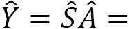
For the example of the four electrons in LiH, with spin pairing (), we derive the following operators from Figure 2.17:

where : is the permutation of particles and , and is the Identity operator.

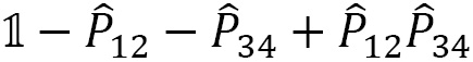
The projection operator is computed using the rules of distributivity and multiplication of permutations:

With this, we will move on to Section 2.2, Postulate 2 – Probability amplitude, where we will revisit the PEP in an example calculation.