Computer vision is a vast field that takes inspiration from many places. Of course, this means that its applications are wide and varied. However, the biggest breakthroughs over the past decade, especially in the context of deep learning applied to visual tasks, have occurred in a particular domain known as image classification.

As the name suggests, image classification consists of the process of discerning what's in an image based on its visual content. Is there a dog or a cat in this image? What number is in this picture? Is the person in this photo smiling or not?

Because image classification is such an important and pervasive task in deep learning applied to computer vision, the recipes in this chapter will focus on the ins and outs of classifying images using TensorFlow 2.x.

We'll cover the following recipes:

• Creating a binary classifier to detect smiles
• Creating a multi-class classifier to play Rock Paper Scissors
• Creating a multi-label classifier to label watches
• Implementing ResNet from scratch
• Classifying images with a pre-trained network using the Keras API
• Classifying images with a pre-trained network using TensorFlow Hub
• Using data augmentation to improve performance with the Keras API
• Using data augmentation to improve performance with the tf.data and tf.image APIs

Besides a working installation of TensorFlow 2.x, it's highly recommended to have access to a GPU, given that some of the recipes are very resource-intensive, making the use of a CPU an inviable option. In each recipe, you'll find the steps and dependencies needed to complete it in the Getting ready section. Finally, the code shown in this chapter is available in full here: https://github.com/PacktPublishing/Tensorflow-2.0-Computer-Vision-Cookbook/tree/master/ch2.

Check out the following link to see the Code in Action video:

https://bit.ly/3bOjqnU

In its most basic form, image classification consists of discerning between two classes, or signaling the presence or absence of some trait. In this recipe, we'll implement a binary classifier that tells us whether a person in a photo is smiling.

Let's begin, shall we?

Getting ready

You'll need to install Pillow, which is very easy with pip:

$> pip install Pillow

We'll use the SMILEs dataset, located here: https://github.com/hromi/SMILEsmileD. Clone or download a zipped version of the repository to a location of your preference. In this recipe, we assume the data is inside the ~/.keras/datasets directory, under the name SMILEsmileD-master:

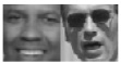
Figure 2.1 – Positive (left) and negative (right) examples

Let's get started!

How to do it…

Follow these steps to train a smile classifier from scratch on the SMILEs dataset:

1. Import all necessary packages:

   import os
   import pathlib
   import glob
   import numpy as np
   from sklearn.model_selection import train_test_split
   from tensorflow.keras import Model
   from tensorflow.keras.layers import *
   from tensorflow.keras.preprocessing.image import *

2. Define a function to load the images and labels from a list of file paths:

   def load_images_and_labels(image_paths):
       images = []
       labels = []
       for image_path in image_paths:
           image = load_img(image_path, target_size=(32,32), 
                            color_mode='grayscale')
           image = img_to_array(image)
           label = image_path.split(os.path.sep)[-2]
           label = 'positive' in label
           label = float(label)
           images.append(image)
           labels.append(label)
       return np.array(images), np.array(labels)

   Notice that we are loading the images in grayscale, and we're encoding the labels by checking whether the word positive is in the file path of the image.

3. Define a function to build the neural network. This model's structure is based on LeNet (you can find a link to LeNet's paper in the See also section):

   def build_network():
       input_layer = Input(shape=(32, 32, 1))
       x = Conv2D(filters=20,
                  kernel_size=(5, 5),
                  padding='same',
                  strides=(1, 1))(input_layer)
       x = ELU()(x)
       x = BatchNormalization()(x)
       x = MaxPooling2D(pool_size=(2, 2),
                        strides=(2, 2))(x)
       x = Dropout(0.4)(x)
       x = Conv2D(filters=50,
                  kernel_size=(5, 5),
                  padding='same',
                  strides=(1, 1))(x)
       x = ELU()(x)
       x = BatchNormalization()(x)
       x = MaxPooling2D(pool_size=(2, 2),
                        strides=(2, 2))(x)
       x = Dropout(0.4)(x)
       x = Flatten()(x)
       x = Dense(units=500)(x)
       x = ELU()(x)
       x = Dropout(0.4)(x)
       output = Dense(1, activation='sigmoid')(x)
       model = Model(inputs=input_layer, outputs=output)
       return model

   Because this is a binary classification problem, a single Sigmoid-activated neuron is enough in the output layer.

4. Load the image paths into a list:

   files_pattern = (pathlib.Path.home() / '.keras' / 
                    'datasets' /
                    'SMILEsmileD-master' / 'SMILEs' / '*' 
                       / '*' / 
                    '*.jpg')
   files_pattern = str(files_pattern)
   dataset_paths = [*glob.glob(files_pattern)]

5. Use the load_images_and_labels() function defined previously to load the dataset into memory:

   X, y = load_images_and_labels(dataset_paths)

6. Normalize the images and compute the number of positive, negative, and total examples in the dataset:

   X /= 255.0
   total = len(y)
   total_positive = np.sum(y)
   total_negative = total - total_positive

7. Create train, test, and validation subsets of the data:

   (X_train, X_test,
    y_train, y_test) = train_test_split(X, y,
                                        test_size=0.2,
                                        stratify=y,
                                        random_state=999)
   (X_train, X_val,
    y_train, y_val) = train_test_split(X_train, y_train,
                                       test_size=0.2,
                                       stratify=y_train,
                                       random_state=999)

8. Instantiate the model and compile it:

   model = build_network()
   model.compile(loss='binary_crossentropy',
                 optimizer='rmsprop',
                 metrics=['accuracy'])

9. Train the model. Because the dataset is unbalanced, we are assigning weights to each class proportional to the number of positive and negative images in the dataset:

   BATCH_SIZE = 32
   EPOCHS = 20
   model.fit(X_train, y_train,
             validation_data=(X_val, y_val),
             epochs=EPOCHS,
             batch_size=BATCH_SIZE,
             class_weight={
                 1.0: total / total_positive,
                 0.0: total / total_negative
             })

10. Evaluate the model on the test set:

    test_loss, test_accuracy = model.evaluate(X_test, 
                                              y_test)

After 20 epochs, the network should get around 90% accuracy on the test set. In the following section, we'll explain the previous steps.

How it works…

We just trained a network to determine whether a person is smiling or not in a picture. Our first big task was to take the images in the dataset and load them into a format suitable for our neural network. Specifically, the load_image_and_labels() function is in charge of loading an image in grayscale, resizing it to 32x32x1, and then converting it into a numpy array. To extract the label, we looked at the containing folder of each image: if it contained the word positive, we encoded the label as 1; otherwise, we encoded it as 0 (a trick we used here was casting a Boolean as a float, like this: float(label)).

Next, we built the neural network, which is inspired by the LeNet architecture. The biggest takeaway here is that because this is a binary classification problem, we can use a single Sigmoid-activated neuron to discern between the two classes.

We then took 20% of the images to comprise our test set, and from the remaining 80% we took an additional 20% to create our validation set. With these three subsets in place, we proceeded to train the network over 20 epochs, using binary_crossentropy as our loss function and rmsprop as the optimizer.

To account for the imbalance in the dataset (out of the 13,165 images, only 3,690 contain smiling people, while the remaining 9,475 do not), we passed a class_weight dictionary where we assigned a weight conversely proportional to the number of instances of each class in the dataset, effectively forcing the model to pay more attention to the 1.0 class, which corresponds to smile.

Finally, we achieved around 90.5% accuracy on the test set.

See also

For more information on the SMILEs dataset, you can visit the official GitHub repository here: https://github.com/hromi/SMILEsmileD. You can read the LeNet paper here (it's pretty long, though): http://yann.lecun.com/exdb/publis/pdf/lecun-98.pdf.

More often than not, we are interested in categorizing an image into more than two classes. As we'll see in this recipe, implementing a neural network to differentiate between many categories is fairly straightforward, and what better way to demonstrate this than by training a model that can play the widely known Rock Paper Scissors game?

Are you ready? Let's dive in!

Getting ready

We'll use the Rock-Paper-Scissors Images dataset, which is hosted on Kaggle at the following location: https://www.kaggle.com/drgfreeman/rockpaperscissors. To download it, you'll need a Kaggle account, so sign in or sign up accordingly. Then, unzip the dataset in a location of your preference. In this recipe, we assume the unzipped folder is inside the ~/.keras/datasets directory, under the name rockpaperscissors.

Here are some sample images:

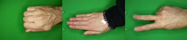
Figure 2.2 – Example images of rock (left), paper (center), and scissors (right)

Let's begin implementing.

How to do it…

The following steps explain how to train a multi-class Convolutional Neural Network (CNN) to distinguish between the three classes of the Rock Paper Scissors game:

1. Import the required packages:

   import os
   import pathlib
   import glob
   import numpy as np
   import tensorflow as tf
   from sklearn.model_selection import train_test_split
   from tensorflow.keras import Model
   from tensorflow.keras.layers import *
   from tensorflow.keras.losses import CategoricalCrossentropy

2. Define a list with the three classes, and also an alias to tf.data.experimental.AUTOTUNE, which we'll use later:

   CLASSES = ['rock', 'paper', 'scissors']
   AUTOTUNE = tf.data.experimental.AUTOTUNE

   The values in CLASSES match the names of the directories that contain the images for each class.

3. Define a function to load an image and its label, given its file path:

   def load_image_and_label(image_path, target_size=(32, 32)):
       image = tf.io.read_file(image_path)
       image = tf.image.decode_jpeg(image, channels=3)
       image = tf.image.rgb_to_grayscale(image)
       image = tf.image.convert_image_dtype(image, 
                                            np.float32)
       image = tf.image.resize(image, target_size)
       label = tf.strings.split(image_path,os.path.sep)[-2]
       label = (label == CLASSES)  # One-hot encode.
       label = tf.dtypes.cast(label, tf.float32)
       return image, label

   Notice that we are one-hot encoding by comparing the name of the folder that contains the image (extracted from image_path) with the CLASSES list.

4. Define a function to build the network architecture. In this case, it's a very simple and shallow one, which is enough for the problem we are solving:

   def build_network():
       input_layer = Input(shape=(32, 32, 1))
       x = Conv2D(filters=32,
                  kernel_size=(3, 3),
                  padding='same',
                  strides=(1, 1))(input_layer)
       x = ReLU()(x)
       x = Dropout(rate=0.5)(x)
       x = Flatten()(x)
       x = Dense(units=3)(x)
       output = Softmax()(x)
       return Model(inputs=input_layer, outputs=output)

5. Define a function to, given a path to a dataset, return a tf.data.Dataset instance of images and labels, in batches and optionally shuffled:

   def prepare_dataset(dataset_path,
                       buffer_size,
                       batch_size,
                       shuffle=True):
       dataset = (tf.data.Dataset
                  .from_tensor_slices(dataset_path)
                  .map(load_image_and_label,
                       num_parallel_calls=AUTOTUNE))
       if shuffle:
           dataset.shuffle(buffer_size=buffer_size)
       dataset = (dataset
                  .batch(batch_size=batch_size)
                  .prefetch(buffer_size=buffer_size))
       return dataset

6. Load the image paths into a list:

   file_patten = (pathlib.Path.home() / '.keras' / 
                  'datasets' /
                  'rockpaperscissors' / 'rps-cv-images' / 
                    '*' /
                  '*.png')
   file_pattern = str(file_patten)
   dataset_paths = [*glob.glob(file_pattern)]

7. Create train, test, and validation subsets of image paths:

   train_paths, test_paths = train_test_split(dataset_paths,
                                             test_size=0.2,
                                           random_state=999)
   train_paths, val_paths = train_test_split(train_paths,
                                         test_size=0.2,
                                        random_state=999)

8. Prepare the training, test, and validation datasets:

   BATCH_SIZE = 1024
   BUFFER_SIZE = 1024
   train_dataset = prepare_dataset(train_paths,
                                 buffer_size=BUFFER_SIZE,
                                   batch_size=BATCH_SIZE)
   validation_dataset = prepare_dataset(val_paths,
                                 buffer_size=BUFFER_SIZE,
                                  batch_size=BATCH_SIZE,
                                   shuffle=False)
   test_dataset = prepare_dataset(test_paths,
                                 buffer_size=BUFFER_SIZE,
                                  batch_size=BATCH_SIZE,
                                  shuffle=False)

9. Instantiate and compile the model:

   model = build_network()
   model.compile(loss=CategoricalCrossentropy
                (from_logits=True),
                 optimizer='adam',
                 metrics=['accuracy'])

10. Fit the model for 250 epochs:

    EPOCHS = 250
    model.fit(train_dataset,
              validation_data=validation_dataset,
              epochs=EPOCHS)

11. Evaluate the model on the test set:

    test_loss, test_accuracy = model.evaluate(test_dataset)

After 250 epochs, our network achieves around 93.5% accuracy on the test set. Let's understand what we just did.

How it works…

We started by defining the CLASSES list, which allowed us to quickly one-hot encode the labels of each image, based on the name of the directory where they were contained, as we observed in the body of the load_image_and_label() function. In this same function, we read an image from disk, decoded it from its JPEG format, converted it to grayscale (color information is not necessary in this problem), and then resized it to more manageable dimensions of 32x32x1.

build_network() creates a very simple and shallow CNN, comprising a single convolutional layer, activated with ReLU(), followed by an output, a fully connected layer of three neurons, corresponding to the number of categories in the dataset. Because this is a multi-class classification task, we use Softmax() to activate the outputs.

prepare_dataset() leverages the load_image_and_label() function defined previously to convert file paths into batches of image tensors and one-hot encoded labels.

Using the three functions explained here, we prepared three subsets of data, with the purpose of training, validating, and testing the neural network. We trained the model for 250 epochs, using the adam optimizer and CategoricalCrossentropy(from_logits=True) as our loss function (from_logits=True produces a bit more numerical stability).

Finally, we got around 93.5% accuracy on the test set. Based on these results, you could use this network as a component of a Rock Paper Scissors game to recognize the hand gestures of a player and react accordingly.

See also

For more information on the Rock-Paper-Scissors Images dataset, refer to the official Kaggle page where it's hosted: https://www.kaggle.com/drgfreeman/rockpaperscissors.

A neural network is not limited to modeling the distribution of a single variable. In fact, it can easily handle instances where each image has multiple labels associated with it. In this recipe, we'll implement a CNN to classify the gender and style/usage of watches.

Let's get started.

Getting ready

First, we must install Pillow:

$> pip install Pillow

Next, we'll use the Fashion Product Images (Small) dataset hosted in Kaggle, which, after signing in, you can download here: https://www.kaggle.com/paramaggarwal/fashion-product-images-small. In this recipe, we assume the data is inside the ~/.keras/datasets directory, under the name fashion-product-images-small. We'll only use a subset of the data, focused on watches, which we'll construct programmatically in the How to do it… section.

Here are some sample images:

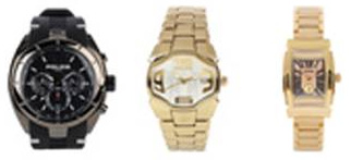
Figure 2.3 – Example images

Let's begin the recipe.

How to do it…

Let's review the steps to complete the recipe:

1. Import the necessary packages:

   import os
   import pathlib
   from csv import DictReader
   import glob
   import numpy as np
   from sklearn.model_selection import train_test_split
   from sklearn.preprocessing import MultiLabelBinarizer
   from tensorflow.keras.layers import *
   from tensorflow.keras.models import Model
   from tensorflow.keras.preprocessing.image import *

2. Define a function to build the network architecture. First, implement the convolutional blocks:

   def build_network(width, height, depth, classes):
       input_layer = Input(shape=(width, height, depth))
       x = Conv2D(filters=32,
                  kernel_size=(3, 3),
                  padding='same')(input_layer)
       x = ReLU()(x)
       x = BatchNormalization(axis=-1)(x)
       x = Conv2D(filters=32,
                  kernel_size=(3, 3),
                  padding='same')(x)
       x = ReLU()(x)
       x = BatchNormalization(axis=-1)(x)
       x = MaxPooling2D(pool_size=(2, 2))(x)
       x = Dropout(rate=0.25)(x)
       x = Conv2D(filters=64,
                  kernel_size=(3, 3),
                  padding='same')(x)
       x = ReLU()(x)
       x = BatchNormalization(axis=-1)(x)
       x = Conv2D(filters=64,
                  kernel_size=(3, 3),
                  padding='same')(x)
       x = ReLU()(x)
       x = BatchNormalization(axis=-1)(x)
       x = MaxPooling2D(pool_size=(2, 2))(x)
       x = Dropout(rate=0.25)(x)

   Next, add the fully convolutional layers:

       x = Flatten()(x)
       x = Dense(units=512)(x)
       x = ReLU()(x)
       x = BatchNormalization(axis=-1)(x)
       x = Dropout(rate=0.5)(x)
       x = Dense(units=classes)(x)
       output = Activation('sigmoid')(x)
       return Model(input_layer, output)

3. Define a function to load all images and labels (gender and usage), given a list of image paths and a dictionary of metadata associated with each of them:

   def load_images_and_labels(image_paths, styles, 
                              target_size):
       images = []
       labels = []
       for image_path in image_paths:
           image = load_img(image_path, 
                            target_size=target_size)
           image = img_to_array(image)
           image_id = image_path.split(os.path.sep)[-
                                            1][:-4]
           image_style = styles[image_id]
           label = (image_style['gender'], 
                    image_style['usage'])
           images.append(image)
           labels.append(label)
       return np.array(images), np.array(labels)

4. Set the random seed to guarantee reproducibility:

   SEED = 999
   np.random.seed(SEED)

5. Define the paths to the images and the styles.csv metadata file:

   base_path = (pathlib.Path.home() / '.keras' / 
                'datasets' /
                'fashion-product-images-small')
   styles_path = str(base_path / 'styles.csv')
   images_path_pattern = str(base_path / 'images/*.jpg')
   image_paths = glob.glob(images_path_pattern)

6. Keep only the Watches images for Casual, Smart Casual, and Formal usage, suited to Men and Women:

   with open(styles_path, 'r') as f:
       dict_reader = DictReader(f)
       STYLES = [*dict_reader]
       article_type = 'Watches'
       genders = {'Men', 'Women'}
       usages = {'Casual', 'Smart Casual', 'Formal'}
       STYLES = {style['id']: style
                 for style in STYLES
                 if (style['articleType'] == article_type 
                                              and
                     style['gender'] in genders and
                     style['usage'] in usages)}
   image_paths = [*filter(lambda p: 
                  p.split(os.path.sep)[-1][:-4]
                                    in STYLES.keys(),
                          image_paths)]

7. Load the images and labels, resizing the images into a 64x64x3 shape:

   X, y = load_images_and_labels(image_paths, STYLES, 
                                 (64, 64))

8. Normalize the images and multi-hot encode the labels:

   X = X.astype('float') / 255.0
   mlb = MultiLabelBinarizer()
   y = mlb.fit_transform(y)

9. Create the train, validation, and test splits:

   (X_train, X_test,
    y_train, y_test) = train_test_split(X, y,
                                        stratify=y,
                                        test_size=0.2,
                                        
                                       random_state=SEED)
   (X_train, X_valid,
    y_train, y_valid) = train_test_split(X_train, y_train,
                                       stratify=y_train,
                                         test_size=0.2,
                                      random_state=SEED)

10. Build and compile the network:

    model = build_network(width=64,
                          height=64,
                          depth=3,
                          classes=len(mlb.classes_))
    model.compile(loss='binary_crossentropy',
                  optimizer='rmsprop',
                  metrics=['accuracy'])

11. Train the model for 20 epochs, in batches of 64 images at a time:

    BATCH_SIZE = 64
    EPOCHS = 20
    model.fit(X_train, y_train,
              validation_data=(X_valid, y_valid),
              batch_size=BATCH_SIZE,
              epochs=EPOCHS)

12. Evaluate the model on the test set:

    result = model.evaluate(X_test, y_test, 
                           batch_size=BATCH_SIZE)
    print(f'Test accuracy: {result[1]}')

    This block prints as follows:

    Test accuracy: 0.90233546

13. Use the model to make predictions on a test image, displaying the probability of each label:

    test_image = np.expand_dims(X_test[0], axis=0)
    probabilities = model.predict(test_image)[0]
    for label, p in zip(mlb.classes_, probabilities):
        print(f'{label}: {p * 100:.2f}%')

    That prints this:

    Casual: 100.00%
    Formal: 0.00%
    Men: 1.08%
    Smart Casual: 0.01%
    Women: 99.16%

14. Compare the ground truth labels with the network's prediction:

    ground_truth_labels = np.expand_dims(y_test[0], 
                                         axis=0)
    ground_truth_labels = mlb.inverse_transform(ground_truth_labels)
    print(f'Ground truth labels: {ground_truth_labels}')

    The output is as follows:

    Ground truth labels: [('Casual', 'Women')]

Let's see how it all works in the next section.

How it works…

We implemented a smaller version of a VGG network, which is capable of performing multi-label, multi-class classification, by modeling independent distributions for the gender and usage metadata associated with each watch. In other words, we modeled two binary classification problems at the same time: one for gender, and one for usage. This is the reason we activated the outputs of the network with Sigmoid, instead of Softmax, and also why the loss function used is binary_crossentropy and not categorical_crossentropy.

We trained the aforementioned network over 20 epochs, on batches of 64 images at a time, obtaining a respectable 90% accuracy on the test set. Finally, we made a prediction on an unseen image from the test set and verified that the labels produced with great certainty by the network (100% certainty for Casual, and 99.16% for Women) correspond to the ground truth categories Casual and Women.

See also

For more information on the Fashion Product Images (Small) dataset, refer to the official Kaggle page where it is hosted: https://www.kaggle.com/paramaggarwal/fashion-product-images-small. I recommend you read the paper where the seminal VGG architecture was introduced: https://arxiv.org/abs/1409.1556.

Residual Network, or ResNet for short, constitutes one of the most groundbreaking advancements in deep learning. This architecture relies on a component called the residual module, which allows us to ensemble networks with depths that were unthinkable a couple of years ago. There are variants of ResNet that have more than 100 layers, without any loss of performance!

In this recipe, we'll implement ResNet from scratch and train it on the challenging drop-in replacement to CIFAR-10, CINIC-10.

Getting ready

We won't explain ResNet in depth, so it is a good idea to familiarize yourself with the architecture if you are interested in the details. You can read the original paper here: https://arxiv.org/abs/1512.03385.

How to do it…

Follow these steps to implement ResNet from the ground up:

1. Import all necessary modules:

   import os
   import numpy as np
   import tarfile
   import tensorflow as tf
   from tensorflow.keras.callbacks import ModelCheckpoint
   from tensorflow.keras.layers import *
   from tensorflow.keras.models import *
   from tensorflow.keras.regularizers import l2
   from tensorflow.keras.utils import get_file

2. Define an alias to the tf.data.expertimental.AUTOTUNE option, which we'll use later:

   AUTOTUNE = tf.data.experimental.AUTOTUNE

3. Define a function to create a residual module in the ResNet architecture. Let's start by specifying the function signature and implementing the first block:

   def residual_module(data,
                       filters,
                       stride,
                       reduce=False,
                       reg=0.0001,
                       bn_eps=2e-5,
                       bn_momentum=0.9):
       bn_1 = BatchNormalization(axis=-1,
                                 epsilon=bn_eps,
                              momentum=bn_momentum)(data)
       act_1 = ReLU()(bn_1)
       conv_1 = Conv2D(filters=int(filters / 4.),
                       kernel_size=(1, 1),
                       use_bias=False,
                       kernel_regularizer=l2(reg))(act_1)

   Let's now implement the second and third blocks:

       bn_2 = BatchNormalization(axis=-1,
                                 epsilon=bn_eps,
                            momentum=bn_momentum)(conv_1)
       act_2 = ReLU()(bn_2)
       conv_2 = Conv2D(filters=int(filters / 4.),
                       kernel_size=(3, 3),
                       strides=stride,
                       padding='same',
                       use_bias=False,
                       kernel_regularizer=l2(reg))(act_2)
       bn_3 = BatchNormalization(axis=-1,
                                 epsilon=bn_eps,
                                 momentum=bn_momentum)(conv_2)
       act_3 = ReLU()(bn_3)
       conv_3 = Conv2D(filters=filters,
                       kernel_size=(1, 1),
                       use_bias=False,
                       kernel_regularizer=l2(reg))(act_3)

   If reduce=True, we apply a 1x1 convolution:

       if reduce:
           shortcut = Conv2D(filters=filters,
                             kernel_size=(1, 1),
                             strides=stride,
                             use_bias=False,
                       kernel_regularizer=l2(reg))(act_1)

   Finally, we combine the shortcut and the third block into a single layer and return that as our output:

       x = Add()([conv_3, shortcut])
       return x

4. Define a function to build a custom ResNet network:

   def build_resnet(input_shape,
                    classes,
                    stages,
                    filters,
                    reg=1e-3,
                    bn_eps=2e-5,
                    bn_momentum=0.9):
       inputs = Input(shape=input_shape)
       x = BatchNormalization(axis=-1,
                              epsilon=bn_eps,
                              
                            momentum=bn_momentum)(inputs)
       x = Conv2D(filters[0], (3, 3),
                  use_bias=False,
                  padding='same',
                  kernel_regularizer=l2(reg))(x)
       for i in range(len(stages)):
           stride = (1, 1) if i == 0 else (2, 2)
           x = residual_module(data=x,
                               filters=filters[i + 1],
                               stride=stride,
                               reduce=True,
                               bn_eps=bn_eps,
                               bn_momentum=bn_momentum)
           for j in range(stages[i] - 1):
               x = residual_module(data=x,
                                   filters=filters[i + 
                                                  1],
                                   stride=(1, 1),
                                   bn_eps=bn_eps,
                                   
                               bn_momentum=bn_momentum)
       x = BatchNormalization(axis=-1,
                              epsilon=bn_eps,
                              momentum=bn_momentum)(x)
       x = ReLU()(x)
       x = AveragePooling2D((8, 8))(x)
       x = Flatten()(x)
       x = Dense(classes, kernel_regularizer=l2(reg))(x)
       x = Softmax()(x)
       return Model(inputs, x, name='resnet')

5. Define a function to load an image and its one-hot encoded labels, based on its file path:

   def load_image_and_label(image_path, target_size=(32, 32)):
       image = tf.io.read_file(image_path)
       image = tf.image.decode_png(image, channels=3)
       image = tf.image.convert_image_dtype(image, 
                                           np.float32)
       image -= CINIC_MEAN_RGB  # Mean normalize
       image = tf.image.resize(image, target_size)
       label = tf.strings.split(image_path, os.path.sep)[-2]
       label = (label == CINIC_10_CLASSES)  # One-hot encode.
       label = tf.dtypes.cast(label, tf.float32)
       return image, label

6. Define a function to create a tf.data.Dataset instance of images and labels from a glob-like pattern that refers to the folder where the images are:

   def prepare_dataset(data_pattern, shuffle=False):
       dataset = (tf.data.Dataset
                  .list_files(data_pattern)
                  .map(load_image_and_label,
                       num_parallel_calls=AUTOTUNE)
                  .batch(BATCH_SIZE))
       
       if shuffle:
           dataset = dataset.shuffle(BUFFER_SIZE)
           
       return dataset.prefetch(BATCH_SIZE)

7. Define the mean RGB values of the CINIC-10 dataset, which is used in the load_image_and_label() function to mean normalize the images (this information is available on the official CINIC-10 site):

   CINIC_MEAN_RGB = np.array([0.47889522, 0.47227842, 0.43047404])

8. Define the classes of the CINIC-10 dataset:

   CINIC_10_CLASSES = ['airplane', 'automobile', 'bird', 'cat',
                       'deer', 'dog', 'frog', 'horse',    'ship',
                       'truck']

9. Download and extract the CINIC-10 dataset to the ~/.keras/datasets directory:

   DATASET_URL = ('https://datashare.is.ed.ac.uk/bitstream/handle/'
                  '10283/3192/CINIC-10.tar.gz?'
                  'sequence=4&isAllowed=y')
   DATA_NAME = 'cinic10'
   FILE_EXTENSION = 'tar.gz'
   FILE_NAME = '.'.join([DATA_NAME, FILE_EXTENSION])
   downloaded_file_location = get_file(origin=DATASET_URL,
                                       fname=FILE_NAME,
                                       extract=False)
   data_directory, _ = (downloaded_file_location
                        .rsplit(os.path.sep, maxsplit=1))
   data_directory = os.path.sep.join([data_directory, 
                                     DATA_NAME])
   tar = tarfile.open(downloaded_file_location)
   if not os.path.exists(data_directory):
       tar.extractall(data_directory)

10. Define the glob-like patterns to the train, test, and validation subsets:

    train_pattern = os.path.sep.join(
        [data_directory, 'train/*/*.png'])
    test_pattern = os.path.sep.join(
        [data_directory, 'test/*/*.png'])
    valid_pattern = os.path.sep.join(
        [data_directory, 'valid/*/*.png'])

11. Prepare the datasets:

    BATCH_SIZE = 128
    BUFFER_SIZE = 1024
    train_dataset = prepare_dataset(train_pattern, 
                                    shuffle=True)
    test_dataset = prepare_dataset(test_pattern)
    valid_dataset = prepare_dataset(valid_pattern)

12. Build, compile, and train a ResNet model. Because this is a time-consuming process, we'll save a version of the model after each epoch, using the ModelCheckpoint() callback:

    model = build_resnet(input_shape=(32, 32, 3),
                         classes=10,
                         stages=(9, 9, 9),
                         filters=(64, 64, 128, 256),
                         reg=5e-3)
    model.compile(loss='categorical_crossentropy',
                  optimizer='rmsprop',
                  metrics=['accuracy'])
    model_checkpoint_callback = ModelCheckpoint(
        filepath='./model.{epoch:02d}-{val_accuracy:.2f}.hdf5',
        save_weights_only=False,
        monitor='val_accuracy')
    EPOCHS = 100
    model.fit(train_dataset,
              validation_data=valid_dataset,
              epochs=EPOCHS,
              callbacks=[model_checkpoint_callback])

13. Load the best model (in this case, model.38-0.72.hdf5) and evaluate it on the test set:

    model = load_model('model.38-0.72.hdf5')
    result = model.evaluate(test_dataset)
    print(f'Test accuracy: {result[1]}')

    This prints the following:

    Test accuracy: 0.71956664

Let's learn how it all works in the next section.

How it works…

The key to ResNet is the residual module, which we implemented in Step 3. A residual module is a micro-architecture that can be reused many times to create a macro-architecture, thus achieving great depths. The residual_module() function receives the input data (data), the number of filters (filters), the stride (stride) of the convolutional blocks, a reduce flag to indicate whether we want to reduce the spatial size of the shortcut branch by applying a 1x1 convolution (a technique used to reduce the dimensionality of the output volumes of the filters), and parameters to adjust the amount of regularization (reg) and batch normalization applied to the different layers (bn_eps and bn_momentum).

A residual module comprises two branches: the first one is the skip connection, also known as the shortcut branch, which is basically the same as the input. The second or main branch is composed of three convolution blocks: a 1x1 with a quarter of the filters, a 3x3 one, also with a quarter of the filters, and finally another 1x1, which uses all the filters. The shortcut and main branches are concatenated in the end using the Add() layer.

build_network() allows us to specify the number of stages to use, and also the number of filters per stage. We start by applying a 3x3 convolution to the input (after being batch normalized). Then we proceed to create the stages. A stage is a series of residual modules connected to each other. The length of the stages list controls the number of stages to create, and each element in this list controls the number of layers in that particular stage. The filters parameter contains the number of filters to use in each residual block within a stage. Finally, we built a fully connected network, Softmax-activated, on top of the stages with as many units as there are classes in the dataset (in this case, 10).

Because ResNet is a very deep, heavy, and slow-to-train architecture, we checkpointed the model after each epoch. In this recipe, we obtained the best model in epoch 38, which produced 72% accuracy on the test set, a respectable performance considering that CINIC-10 is not an easy dataset and that we did not apply any data augmentation or transfer learning.

See also

For more information on the CINIC-10 dataset, visit this link: https://datashare.is.ed.ac.uk/handle/10283/3192.

We do not always need to train a classifier from scratch, especially when the images we want to categorize resemble ones that another network trained on. In these instances, we can simply reuse the model, saving ourselves lots of time. In this recipe, we'll use a pre-trained network on ImageNet to classify a custom image.

Let's begin!

Getting ready

We will need Pillow. We can install it as follows:

$> pip install Pillow

You're free to use your own images in the recipe. Alternatively, you can download the one at this link: https://github.com/PacktPublishing/Tensorflow-2.0-Computer-Vision-Cookbook/tree/master/ch2/recipe5/dog.jpg.

Here's the image we'll pass to the classifier:

Figure 2.4 – Image passed to the pre-trained classifier

How to do it…

As we'll see in this section, re-using a pre-trained classifier is very easy!

1. Import the required packages. These include the pre-trained network used for classification, as well as some helper functions to pre process the images:

   import matplotlib.pyplot as plt
   import numpy as np
   from tensorflow.keras.applications import imagenet_utils
   from tensorflow.keras.applications.inception_v3 import *
   from tensorflow.keras.preprocessing.image import *

2. Instantiate an InceptionV3 network pre-trained on ImageNet:

   model = InceptionV3(weights='imagenet')

3. Load the image to classify. InceptionV3 takes a 299x299x3 image, so we must resize it accordingly:

   image = load_img('dog.jpg', target_size=(299, 299))

4. Convert the image to a numpy array, and wrap it into a singleton batch:

   image = img_to_array(image)
   image = np.expand_dims(image, axis=0)

5. Pre process the image the same way InceptionV3 does:

   image = preprocess_input(image)

6. Use the model to make predictions on the image, and then decode the predictions to a matrix:

   predictions = model.predict(image)
   prediction_matrix = (imagenet_utils
                        .decode_predictions(predictions))

7. Examine the top 5 predictions along with their probability:

   for i in range(5):
       _, label, probability = prediction_matrix[0][i]
       print(f'{i + 1}. {label}: {probability * 100:.3f}%')

   This produces the following output:

   1. pug: 85.538%
   2. French_bulldog: 0.585%
   3. Brabancon_griffon: 0.543%
   4. Boston_bull: 0.218%
   5. bull_mastiff: 0.125%

8. Plot the original image with its most probable label:

   _, label, _ = prediction_matrix[0][0]
   plt.figure()
   plt.title(f'Label: {label}.')
   original = load_img('dog.jpg')
   original = img_to_array(original)
   plt.imshow(original / 255.0)
   plt.show()

   This block generates the following image:

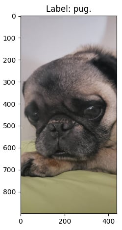
Figure 2.5 – Correctly classified image

Let's see how it all works in the next section.

How it works…

As evidenced here, in order to classify images effortlessly, using a pre-trained network on ImageNet, we just need to instantiate the proper model with the right weights, like this: InceptionV3(weights='imagenet'). This will download the architecture and the weights if it is the first time we are using them; otherwise, a version of these files will be cached in our system.

Then, we loaded the image we wanted to classify, resized it to dimensions compatible with InceptionV3 (299x299x3), converted it into a singleton batch with np.expand_dims(image, axis=0), and pre processed it the same way InceptionV3 did when it was trained, with preprocess_input(image).

Next, we got the predictions from the model, which we need to transform to a prediction matrix with the help of imagenet_utils.decode_predictions(predictions). This matrix contains the label and probabilities in the 0th row, which we inspected to get the five most probable classes.

See also

You can read more about Keras pre-trained models here: https://www.tensorflow.org/api_docs/python/tf/keras/applications.

TensorFlow Hub (TFHub) is a repository of hundreds of machine learning models contributed to by the big and rich community that surrounds TensorFlow. Here we can find models for a myriad of different tasks, not only for computer vision but for applications in many different domains, such as Natural Language Processing (NLP) and reinforcement learning.

In this recipe, we'll use a model trained on ImageNet, hosted on TFHub, to make predictions on a custom image. Let's begin!

Getting ready

We'll need the tensorflow-hub and Pillow packages, which can be easily installed using pip, as follows:

$> pip install tensorflow-hub Pillow

If you want to use the same image we use in this recipe, you can download it here: https://github.com/PacktPublishing/Tensorflow-2.0-Computer-Vision-Cookbook/tree/master/ch2/recipe6/beetle.jpg.

Here's the image we'll classify:

Figure 2.6 – Image to be classified

Let's head to the next section.

How to do it…

Let's proceed with the recipe steps:

1. Import the necessary packages:

   import matplotlib.pyplot as plt
   import numpy as np
   import tensorflow_hub as hub
   from tensorflow.keras import Sequential
   from tensorflow.keras.preprocessing.image import *
   from tensorflow.keras.utils import get_file

2. Define the URL of the pre-trained ResNetV2152 classifier in TFHub:

   classifier_url = ('https://tfhub.dev/google/imagenet/'
                     'resnet_v2_152/classification/4')

3. Download and instantiate the classifier hosted on TFHub:

   model = Sequential([
       hub.KerasLayer(classifier_url, input_shape=(224, 
                                                 224, 3))])

4. Load the image we'll classify, convert it to a numpy array, normalize it, and wrap it into a singleton batch:

   image = load_img('beetle.jpg', target_size=(224, 224))
   image = img_to_array(image)
   image = image / 255.0
   image = np.expand_dims(image, axis=0)

5. Use the pre-trained model to classify the image:

   predictions = model.predict(image)

6. Extract the index of the most probable prediction:

   predicted_index = np.argmax(predictions[0], axis=-1)

7. Download the ImageNet labels into a file named ImageNetLabels.txt:

   file_name = 'ImageNetLabels.txt'
   file_url = ('https://storage.googleapis.com/'
       'download.tensorflow.org/data/ImageNetLabels.txt')
            labels_path = get_file(file_name, file_url)

8. Read the labels into a numpy array:

   with open(labels_path) as f:
       imagenet_labels = np.array(f.read().splitlines())

9. Extract the name of the class corresponding to the index of the most probable prediction:

   predicted_class = imagenet_labels[predicted_index]

10. Plot the original image with its most probable label:

    plt.figure()
    plt.title(f'Label: {predicted_class}.')
    original = load_img('beetle.jpg')
    original = img_to_array(original)
    plt.imshow(original / 255.0)
    plt.show()

    This produces the following:

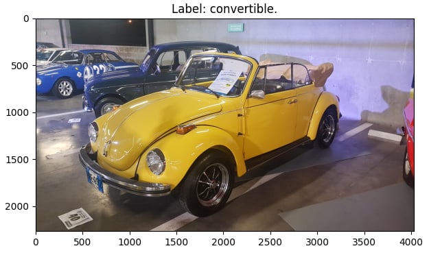
Figure 2.7 – Correctly classified image

Let's see how it all works.

How it works…

After importing the relevant packages, we proceeded to define the URL of the model we wanted to use to classify our input image. To download and convert such a network into a Keras model, we used the convenient hub.KerasLayer class in Step 3. Then, in Step 4, we loaded the image we wanted to classify into memory, making sure its dimensions match the ones the network expects: 224x224x3.

Steps 5 and 6 perform the classification and extract the most probable category, respectively. However, to make this prediction human-readable, we downloaded a plain text file with all ImageNet labels in Step 7, which we then parsed using numpy, allowing us to use the index of the most probable category to obtain the corresponding label, finally displayed in Step 10 along with the input image.

See also

You can learn more about the pre-trained model we used here: https://tfhub.dev/google/imagenet/resnet_v2_152/classification/4.

More often than not, we can benefit from providing more data to our model. But data is expensive and scarce. Is there a way to circumvent this limitation? Yes, there is! We can synthesize new training examples by performing little modifications on the ones we already have, such as random rotations, random cropping, and horizontal flipping, among others. In this recipe, we'll learn how to use data augmentation with the Keras API to improve performance.

Let's begin.

Getting ready

We must install Pillow and tensorflow_docs:

$> pip install Pillow git+https://github.com/tensorflow/docs

In this recipe, we'll use the Caltech 101 dataset, which is available here: http://www.vision.caltech.edu/Image_Datasets/Caltech101/. Download and decompress 101_ObjectCategories.tar.gz to your preferred location. From now on, we assume the data is inside the ~/.keras/datasets directory, under the name 101_ObjectCategories.

Here are sample images from Caltech 101:

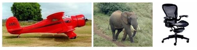
Figure 2.8 – Caltech 101 sample images

Let's implement!

How to do it…

The steps listed here are necessary to complete the recipe. Let's get started!

1. Import the required modules:

   import os
   import pathlib
   import matplotlib.pyplot as plt
   import numpy as np
   import tensorflow_docs as tfdocs
   import tensorflow_docs.plots
   from glob import glob
   from sklearn.model_selection import train_test_split
   from sklearn.preprocessing import LabelBinarizer
   from tensorflow.keras.layers import *
   from tensorflow.keras.models import Model
   from tensorflow.keras.preprocessing.image import *

2. Define a function to load all images in the dataset, along with their labels, based on their file paths:

   def load_images_and_labels(image_paths, target_size=(64, 64)):
       images = []
       labels = []
       for image_path in image_paths:
           image = load_img(image_path, 
                            target_size=target_size)
           image = img_to_array(image)
           label = image_path.split(os.path.sep)[-2]
           images.append(image)
           labels.append(label)
       return np.array(images), np.array(labels)

3. Define a function to build a smaller version of VGG:

   def build_network(width, height, depth, classes):
       input_layer = Input(shape=(width, height, depth))
       x = Conv2D(filters=32,
                  kernel_size=(3, 3),
                  padding='same')(input_layer)
       x = ReLU()(x)
       x = BatchNormalization(axis=-1)(x)
       x = Conv2D(filters=32,
                  kernel_size=(3, 3),
                  padding='same')(x)
       x = ReLU()(x)
       x = BatchNormalization(axis=-1)(x)
       x = MaxPooling2D(pool_size=(2, 2))(x)
       x = Dropout(rate=0.25)(x)
       x = Conv2D(filters=64,
                  kernel_size=(3, 3),
                  padding='same')(x)
       x = ReLU()(x)
       x = BatchNormalization(axis=-1)(x)
       x = Conv2D(filters=64,
                  kernel_size=(3, 3),
                  padding='same')(x)
       x = ReLU()(x)
       x = BatchNormalization(axis=-1)(x)
       x = MaxPooling2D(pool_size=(2, 2))(x)
       x = Dropout(rate=0.25)(x)
       x = Flatten()(x)
       x = Dense(units=512)(x)
       x = ReLU()(x)
       x = BatchNormalization(axis=-1)(x)
       x = Dropout(rate=0.25)(x)
       x = Dense(units=classes)(x)
       output = Softmax()(x)
       return Model(input_layer, output)

4. Define a function to plot and save a model's training curve:

   def plot_model_history(model_history, metric, 
                          plot_name):
       plt.style.use('seaborn-darkgrid')
       plotter = tfdocs.plots.HistoryPlotter()
       plotter.plot({'Model': model_history}, 
                     metric=metric)
       plt.title(f'{metric.upper()}')
       plt.ylim([0, 1])
       plt.savefig(f'{plot_name}.png')
       plt.close()

5. Set the random seed:

   SEED = 999
   np.random.seed(SEED)

6. Load the paths to all images in the dataset, excepting the ones of the BACKGROUND_Google class:

   base_path = (pathlib.Path.home() / '.keras' / 
                'datasets' /
                '101_ObjectCategories')
   images_pattern = str(base_path / '*' / '*.jpg')
   image_paths = [*glob(images_pattern)]
   image_paths = [p for p in image_paths if
                  p.split(os.path.sep)[-2] !=
                 'BACKGROUND_Google']

7. Compute the set of classes in the dataset:

   classes = {p.split(os.path.sep)[-2] for p in 
             image_paths}

8. Load the dataset into memory, normalizing the images and one-hot encoding the labels:

   X, y = load_images_and_labels(image_paths)
   X = X.astype('float') / 255.0
   y = LabelBinarizer().fit_transform(y)

9. Create the training and testing subsets:

   (X_train, X_test,
    y_train, y_test) = train_test_split(X, y,
                                        test_size=0.2,
                                       random_state=SEED)

10. Build, compile, train, and evaluate a neural network without data augmentation:

    EPOCHS = 40
    BATCH_SIZE = 64
    model = build_network(64, 64, 3, len(classes))
    model.compile(loss='categorical_crossentropy',
                  optimizer='rmsprop',
                  metrics=['accuracy'])
    history = model.fit(X_train, y_train,
                        validation_data=(X_test, y_test),
                        epochs=EPOCHS,
                        batch_size=BATCH_SIZE)
    result = model.evaluate(X_test, y_test)
    print(f'Test accuracy: {result[1]}')
    plot_model_history(history, 'accuracy', 'normal')

    The accuracy on the test set is as follows:

    Test accuracy: 0.61347926

    And here's the accuracy curve:

    

    Figure 2.9 – Training and validation accuracy for a network without data augmentation

11. Build, compile, train, and evaluate the same network, this time with data augmentation:

    model = build_network(64, 64, 3, len(classes))
    model.compile(loss='categorical_crossentropy',
                  optimizer='rmsprop',
                  metrics=['accuracy'])
    augmenter = ImageDataGenerator(horizontal_flip=True,
                                   rotation_range=30,
                                   width_shift_range=0.1,
                                   height_shift_range=0.1,
                                   shear_range=0.2,
                                   zoom_range=0.2,
                                   fill_mode='nearest')
    train_generator = augmenter.flow(X_train, y_train, 
                                      BATCH_SIZE)
    hist = model.fit(train_generator,
                     steps_per_epoch=len(X_train) // 
                     BATCH_SIZE,
                     validation_data=(X_test, y_test),
                     epochs=EPOCHS)
    result = model.evaluate(X_test, y_test)
    print(f'Test accuracy: {result[1]}')
    plot_model_history(hist, 'accuracy', 'augmented')

    The accuracy on the test set when we use data augmentation is as follows:

    Test accuracy: 0.65207374

    And the accuracy curve looks like this:

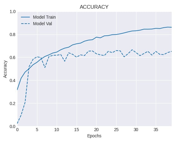
Figure 2.10 – Training and validation accuracy for a network with data augmentation

Comparing Steps 10 and 11, we observe a noticeable gain in performance by using data augmentation. Let's understand better what we did in the next section.

How it works…

In this recipe, we implemented a scaled-down version of VGG on the challenging Caltech 101 dataset. First, we trained a network only on the original data, and then using data augmentation. The first network (see Step 10) obtained an accuracy level on the test set of 61.3% and clearly shows signs of overfitting, because the gap that separates the training and validation accuracy curves is very wide. On the other hand, by applying a series of random perturbations, through ImageDataGenerator(), such as horizontal flips, rotations, width, and height shifting, among others (see Step 11), we increased the accuracy on the test set to 65.2%. Also, the gap between the training and validation accuracy curves is much smaller this time, which suggests a regularization effect resulting from the application of data augmentation.

See also

You can learn more about Caltech 101 here: http://www.vision.caltech.edu/Image_Datasets/Caltech101/.

Data augmentation is a powerful technique we can apply to artificially increment the size of our dataset, by creating slightly modified copies of the images at our disposal. In this recipe, we'll leverage the tf.data and tf.image APIs to increase the performance of a CNN trained on the challenging Caltech 101 dataset.

Getting ready

We must install tensorflow_docs:

$> pip install git+https://github.com/tensorflow/docs

In this recipe, we'll use the Caltech 101 dataset, which is available here: http://www.vision.caltech.edu/Image_Datasets/Caltech101/. Download and decompress 101_ObjectCategories.tar.gz to your preferred location. From now on, we assume the data is inside the ~/.keras/datasets directory, in a folder named 101_ObjectCategories.

Here are some sample images from Caltech 101:

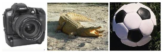
Figure 2.11 – Caltech 101 sample images

Let's go to the next section.

How to do it…

Let's go over the steps required to complete this recipe.

1. Import the necessary dependencies:

   import os
   import pathlib
   import matplotlib.pyplot as plt
   import numpy as np
   import tensorflow as tf
   import tensorflow_docs as tfdocs
   import tensorflow_docs.plots
   from glob import glob
   from sklearn.model_selection import train_test_split
   from tensorflow.keras.layers import *
   from tensorflow.keras.models import Model

2. Create an alias for the tf.data.experimental.AUTOTUNE flag, which we'll use later on:

   AUTOTUNE = tf.data.experimental.AUTOTUNE

3. Define a function to create a smaller version of VGG. Start by creating the input layer and the first block of two convolutions with 32 filters each:

   def build_network(width, height, depth, classes):
       input_layer = Input(shape=(width, height, depth))
       x = Conv2D(filters=32,
                  kernel_size=(3, 3),
                  padding='same')(input_layer)
       x = ReLU()(x)
       x = BatchNormalization(axis=-1)(x)
       x = Conv2D(filters=32,
                  kernel_size=(3, 3),
                  padding='same')(x)
       x = ReLU()(x)
       x = BatchNormalization(axis=-1)(x)
       x = MaxPooling2D(pool_size=(2, 2))(x)
       x = Dropout(rate=0.25)(x)

4. Continue with the second block of two convolutions, this time each with 64 kernels:

       x = Conv2D(filters=64,
                  kernel_size=(3, 3),
                  padding='same')(x)
       x = ReLU()(x)
       x = BatchNormalization(axis=-1)(x)
       x = Conv2D(filters=64,
                  kernel_size=(3, 3),
                  padding='same')(x)
       x = ReLU()(x)
       x = BatchNormalization(axis=-1)(x)
       x = MaxPooling2D(pool_size=(2, 2))(x)
       x = Dropout(rate=0.25)(x)

5. Define the last part of the architecture, which consists of a series of fully connected layers:

       x = Flatten()(x)
       x = Dense(units=512)(x)
       x = ReLU()(x)
       x = BatchNormalization(axis=-1)(x)
       x = Dropout(rate=0.5)(x)
       x = Dense(units=classes)(x)
       output = Softmax()(x)
       return Model(input_layer, output)

6. Define a function to plot and save the training curves of a model, given its training history:

   def plot_model_history(model_history, metric, 
                          plot_name):
       plt.style.use('seaborn-darkgrid')
       plotter = tfdocs.plots.HistoryPlotter()
       plotter.plot({'Model': model_history}, 
                     metric=metric)
       plt.title(f'{metric.upper()}')
       plt.ylim([0, 1])
       plt.savefig(f'{plot_name}.png')
       plt.close()

7. Define a function to load an image and one-hot encode its label, based on the image's file path:

   def load_image_and_label(image_path, target_size=(64, 
                                                    64)):
       image = tf.io.read_file(image_path)
       image = tf.image.decode_jpeg(image, channels=3)
       image = tf.image.convert_image_dtype(image, 
                                            np.float32)
       image = tf.image.resize(image, target_size)
       label = tf.strings.split(image_path, os.path.sep)[-2]
       label = (label == CLASSES)  # One-hot encode.
       label = tf.dtypes.cast(label, tf.float32)
       return image, label

8. Define a function to augment an image by performing random transformations on it:

   def augment(image, label):
       image = tf.image.resize_with_crop_or_pad(image, 
                                                74, 74)
       image = tf.image.random_crop(image, size=(64, 64, 3))
       image = tf.image.random_flip_left_right(image)
       image = tf.image.random_brightness(image, 0.2)
       return image, label

9. Define a function to prepare a tf.data.Dataset of images, based on a glob-like pattern that refers to the folder where they live:

   def prepare_dataset(data_pattern):
       return (tf.data.Dataset
               .from_tensor_slices(data_pattern)
               .map(load_image_and_label,
                    num_parallel_calls=AUTOTUNE))

10. Set the random seed:

    SEED = 999
    np.random.seed(SEED)

11. Load the paths to all images in the dataset, excepting the ones of the BACKGROUND_Google class:

    base_path = (pathlib.Path.home() / '.keras' / 
                 'datasets' /
                 '101_ObjectCategories')
    images_pattern = str(base_path / '*' / '*.jpg')
    image_paths = [*glob(images_pattern)]
    image_paths = [p for p in image_paths if
                   p.split(os.path.sep)[-2] !=
                  'BACKGROUND_Google']

12. Compute the unique categories in the dataset:

    CLASSES = np.unique([p.split(os.path.sep)[-2]
                         for p in image_paths])

13. Split the image paths into training and testing subsets:

    train_paths, test_paths = train_test_split(image_paths,
                                              test_size=0.2,
                                          random_state=SEED)

14. Prepare the training and testing datasets, without augmentation:

    BATCH_SIZE = 64
    BUFFER_SIZE = 1024
    train_dataset = (prepare_dataset(train_paths)
                     .batch(BATCH_SIZE)
                     .shuffle(buffer_size=BUFFER_SIZE)
                     .prefetch(buffer_size=BUFFER_SIZE))
    test_dataset = (prepare_dataset(test_paths)
                    .batch(BATCH_SIZE)
                    .prefetch(buffer_size=BUFFER_SIZE))

15. Instantiate, compile, train and evaluate the network:

    EPOCHS = 40
    model = build_network(64, 64, 3, len(CLASSES))
    model.compile(loss='categorical_crossentropy',
                  optimizer='rmsprop',
                  metrics=['accuracy'])
    history = model.fit(train_dataset,
                        validation_data=test_dataset,
                        epochs=EPOCHS)
    result = model.evaluate(test_dataset)
    print(f'Test accuracy: {result[1]}')
    plot_model_history(history, 'accuracy', 'normal')

    The accuracy on the test set is:

    Test accuracy: 0.6532258

    And here's the accuracy curve:

    

    Figure 2.12 – Training and validation accuracy for a network without data augmentation

16. Prepare the training and testing sets, this time applying data augmentation to the training set:

    train_dataset = (prepare_dataset(train_paths)
                     .map(augment, 
                         num_parallel_calls=AUTOTUNE)
                     .batch(BATCH_SIZE)
                     .shuffle(buffer_size=BUFFER_SIZE)
                     .prefetch(buffer_size=BUFFER_SIZE))
    test_dataset = (prepare_dataset(test_paths)
                    .batch(BATCH_SIZE)
                    .prefetch(buffer_size=BUFFER_SIZE))

17. Instantiate, compile, train, and evaluate the network on the augmented data:

    model = build_network(64, 64, 3, len(CLASSES))
    model.compile(loss='categorical_crossentropy',
                  optimizer='rmsprop',
                  metrics=['accuracy'])
    history = model.fit(train_dataset,
                        validation_data=test_dataset,
                        epochs=EPOCHS)
    result = model.evaluate(test_dataset)
    print(f'Test accuracy: {result[1]}')
    plot_model_history(history, 'accuracy', 'augmented')

    The accuracy on the test set when we use data augmentation is as follows:

    Test accuracy: 0.74711984

    And the accuracy curve looks like this:

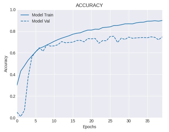
Figure 2.13 – Training and validation accuracy for a network with data augmentation

Let's understand what we just did in the next section.

How it works…

We just implemented a trimmed down version of the famous VGG architecture, trained on the Caltech 101 dataset. To better understand the advantages of data augmentation, we fitted a first version on the original data, without any modification, obtaining an accuracy level of 65.32% on the test set. This first model displays signs of overfitting, because the gap that separates the training and validation accuracy curves widens early in the training process.

Next, we trained the same network on an augmented dataset (see Step 15), using the augment() function defined earlier. This greatly improved the model's performance, reaching a respectable accuracy of 74.19% on the test set. Also, the gap between the training and validation accuracy curves is noticeably smaller, which suggests a regularization effect coming out from the application of data augmentation.

See also

You can learn more about Caltech 101 here: http://www.vision.caltech.edu/Image_Datasets/Caltech101/.