

In order to work effectively with high-dimensional datasets, it is important to have a set of techniques that can reduce this dimensionality down to manageable levels. The advantages of this dimensionality reduction include the ability to plot multivariate data in two dimensions, capture the majority of a dataset's informational content within a minimal number of features, and, in some contexts, identify collinear model components.
Note
For those in need of a refresher, collinearity in a machine learning context refers to model features that share an approximately linear relationship. For reasons that will likely be obvious, these features tend to be unhelpful as the related features are unlikely to add information mutually that either one provides independently. Moreover, collinear features may emphasize local minima or other false leads.
Probably the most widely-used dimensionality reduction technique today is PCA. As we'll be applying PCA in multiple contexts throughout this book, it's appropriate for us to review the technique, understand the theory behind it, and write Python code to effectively apply it.
PCA is a powerful decomposition technique; it allows one to break down a highly multivariate dataset into a set of orthogonal components. When taken together in sufficient number, these components can explain almost all of the dataset's variance. In essence, these components deliver an abbreviated description of the dataset. PCA has a broad set of applications and its extensive utility makes it well worth our time to cover.
Note
Note the slightly cautious phrasing here—a given set of components of length less than the number of variables in the original dataset will almost always lose some amount of the information content within the source dataset. This lossiness is typically minimal, given enough components, but in cases where small numbers of principal components are composed from very high-dimensional datasets, there may be substantial lossiness. As such, when performing PCA, it is always appropriate to consider how many components will be necessary to effectively model the dataset in question.
PCA works by successively identifying the axis of greatest variance in a dataset (the principal components). It does this as follows:
Let's unpack these concepts briefly:
Covariance is effectively variance applied to multiple dimensions; it is the variance between two or more variables. While a single value can capture the variance in one dimension or variable, it is necessary to use a 2 x 2 matrix to capture the covariance between two variables, a 3 x 3 matrix to capture the covariance between three variables, and so on. So the first step in PCA is to calculate this covariance matrix.
An Eigenvector is a vector that is specific to a dataset and linear transformation. Specifically, it is the vector that does not change in direction before and after the transformation is performed. To get a better feeling for how this works, imagine that you're holding a rubber band, straight, between both hands. Let's say you stretch the band out until it is taut between your hands. The eigenvector is the vector that did not change direction between before the stretch and during it; in this case, it's the vector running directly through the center of the band from one hand to the other.
Orthogonalization is the process of finding two vectors that are orthogonal (at right angles) to one another. In an n-dimensional data space, the process of orthogonalization takes a set of vectors and yields a set of orthogonal vectors.
Orthonormalization is an orthogonalization process that also normalizes the product.
Eigenvalue (roughly corresponding to the length of the eigenvector) is used to calculate the proportion of variance represented by each eigenvector. This is done by dividing the eigenvalue for each eigenvector by the sum of eigenvalues for all eigenvectors.
In summary, the covariance matrix is used to calculate Eigenvectors. An orthonormalization process is undertaken that produces orthogonal, normalized vectors from the Eigenvectors. The eigenvector with the greatest eigenvalue is the first principal component with successive components having smaller eigenvalues. In this way, the PCA algorithm has the effect of taking a dataset and transforming it into a new, lower-dimensional coordinate system.
Now that we've reviewed the PCA algorithm at a high level, we're going to jump straight in and apply PCA to a key Python dataset—the UCI handwritten digits dataset, distributed as part of
scikit-learn.
This dataset is composed of 1,797 instances of handwritten digits gathered from 44 different writers. The input (pressure and location) from these authors' writing is resampled twice across an 8 x 8 grid so as to yield maps of the kind shown in the following image:
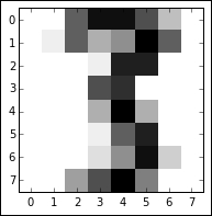
These maps can be transformed into feature vectors of length 64, which are then readily usable as analysis input. With an input dataset of 64 features, there is an immediate appeal to using a technique like PCA to reduce the set of variables to a manageable amount. As it currently stands, we cannot effectively explore the dataset with exploratory visualization!
We will begin applying PCA to the handwritten digits dataset with the following code:
import numpy as np
from sklearn.datasets import load_digits
import matplotlib.pyplot as plt
from sklearn.decomposition import PCA
from sklearn.preprocessing import scale
from sklearn.lda import LDA
import matplotlib.cm as cm

digits = load_digits()
data = digits.data

n_samples, n_features = data.shape
n_digits = len(np.unique(digits.target))
labels = digits.target
This code does several things for us:
First, it loads up a set of necessary libraries, including
numpy, a set of components from scikit-learn, including thedigitsdataset itself, PCA and data scaling functions, and the plotting capability of matplotlib.The code then begins preparing the
digitsdataset. It does several things in order:First, it loads the dataset before creating helpful variables
The
datavariable is created for subsequent use, and the number of distinctdigitsin thetargetvector (0 through to 9, son_digits = 10) is saved as a variable that we can easily access for subsequent analysisThe
targetvector is also saved as labels for later useAll of this variable creation is intended to simplify subsequent analysis
With the dataset ready, we can initialize our PCA algorithm and apply it to the dataset:
pca = PCA(n_components=10)
data_r = pca.fit(data).transform(data)

print('explained variance ratio (first two components): %s' % str(pca.explained_variance_ratio_))
print('sum of explained variance (first two components): %s' % str(sum(pca.explained_variance_ratio_)))
This code outputs the variance explained by each of the first ten principal components ordered by explanatory power.
In the case of this set of 10 principal components, they collectively explain 0.589 of the overall dataset variance. This isn't actually too bad, considering that it's a reduction from 64 variables to 10 components. It does, however, illustrate the potential lossiness of PCA. The key question, though, is whether this reduced set of components makes subsequent analysis or classification easier to achieve; that is, whether many of the remaining components contained variance that disrupts classification attempts.
Having created a data_r object containing the output of pca performed over the digits dataset, let's visualize the output. To do so, we'll first create a vector of colors for class coloration. We then simply create a scatterplot with colorized classes:
X = np.arange(10)
ys = [i+x+(i*x)**2 for i in range(10)]

plt.figure()
colors = cm.rainbow(np.linspace(0, 1, len(ys)))
for c, i target_name in zip(colors, [1,2,3,4,5,6,7,8,9,10], labels):
   plt.scatter(data_r[labels == I, 0], data_r[labels == I, 1],
   c=c, alpha = 0.4)
   plt.legend()
   plt.title('Scatterplot of Points plotted in first \n'
   '10 Principal Components')
   plt.show()
The resulting scatterplot looks as follows:
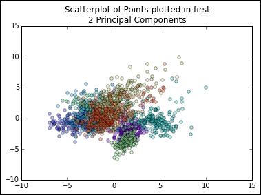
This plot shows us that, while there is some separation between classes in the first two principal components, it may be tricky to classify highly accurately with this dataset. However, classes do appear to be clustered and we may be able to get reasonably good results by employing a clustering analysis. In this way, PCA has given us some insight into how the dataset is structured and has informed our subsequent analysis.
At this point, let's take this insight and move on to examine clustering by the application of the k-means clustering algorithm.