

Now that all of the preliminary things are out of the way, we will code our first extremely simple predictive model. There will be two scripts written to accomplish this.
Our first R script is not a predictive model (yet), but it is a preliminary program which will view and plot some data. The dataset we will use is already built into the R package system, and is not necessary to load externally. For quickly illustrating techniques, I will sometimes use sample data contained within specific R packages themselves in order to demonstrate ideas, rather than pulling data in from an external file.
In this case our data will be pulled from the datasets package, which is loaded by default at startup.
- Paste the following code into the
Untitled1scripts that was just created. Dont worry about what each line means yet. I will cover the specific lines after the code is executed:
        require(graphics)
        data(women)
        head(women)
        View(women)
plot(women$height,women$weight)- Within the code pane, you will see a menu bar right beneath the
Untitled1tab. It should look something like this:

- To execute the code, Click the
Sourceicon. The display should then change to the following diagram:
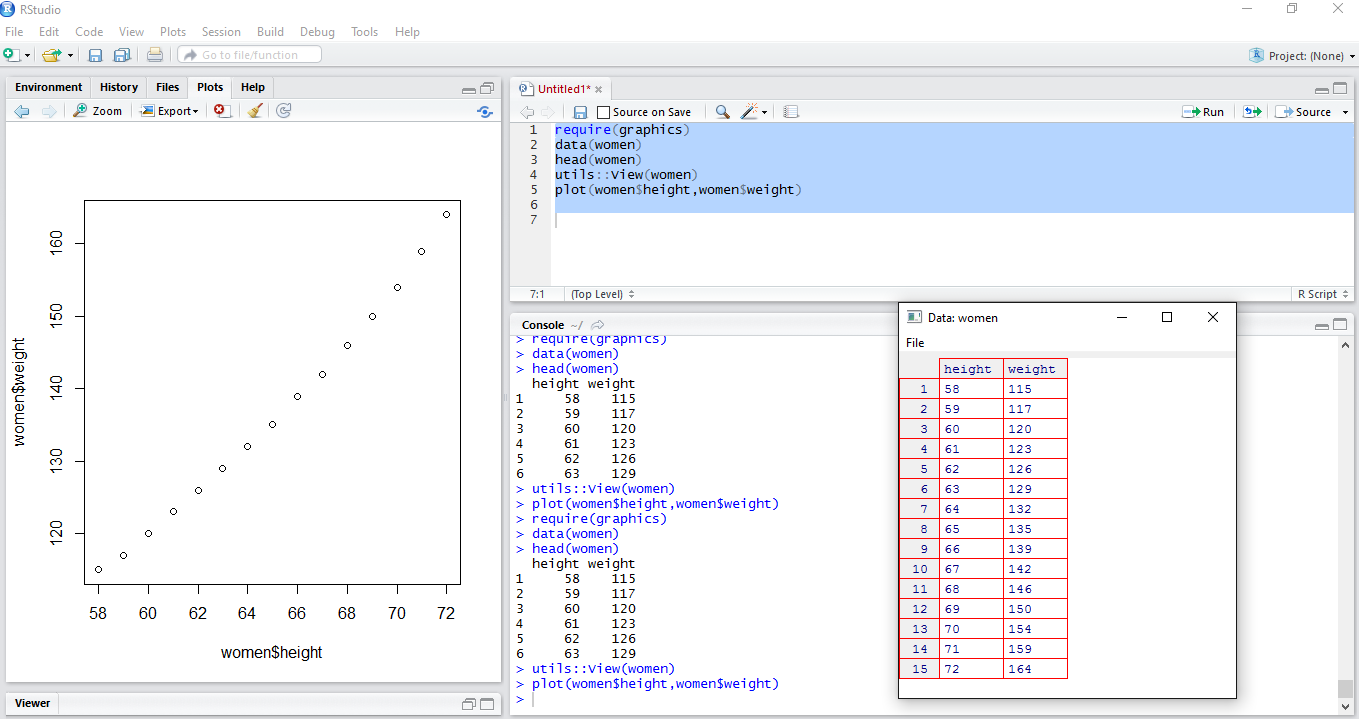
Notice from the preceding picture that three things have changed:
- Output has been written to the
Consolepane. - The
Viewpane has popped up which contains a two column table. - Additionally, a plot will appear in the
Plotpane.
Here are some more details on what the code has accomplished:
- Line 1 of the code contains the function
require, which is just a way of saying that R needs a specific package to run. In this caserequire(graphics)specifies that thegraphicspackage is needed for the analysis, and it will load it into memory. If it is not available, you will get an error message. However,graphicsis a base package and should be available. - Line 2 of the code loads the
Womendata object into memory using thedata(women)function. - Lines 3-5 of the code display the raw data in three different ways:
View(women): This will visually display the DataFrame. Although this is part of the actual R script, viewing a DataFrame is a very common task, and is often issued directly as a command via the R Console. As you can see in the previous figure , theWomendataframe has 15 rows, and 2 columns namedheightandweight.plot(women$height,women$weight): This uses the native Rplotfunction, which plots the values of the two variables against each other. It is usually the first step one does to begin to understand the relationship between two variables. As you can see, the relationship is very linear.head(women): This displays the first N rows of theWomendataframe to the console. If you want no more than a certain number of rows, add that as a second argument of the function. For example,Head(women,99)will display up to 99 rows in the console. Thetail()function works similarly, but displays the last rows of data.
Note
The utils:View(women) function can also be shortened to just View(women). I have added the prefix utils:: to indicate that the View() function is part of the utils package. There is generally no reason to add the prefix unless there is a function name conflict. This can happen when you have identically named functions sourced from two different packages which are loaded in memory. We will see these kind of function name conflicts in later chapters. But it is always safe to prefix a function name with the name of the package that it comes from.