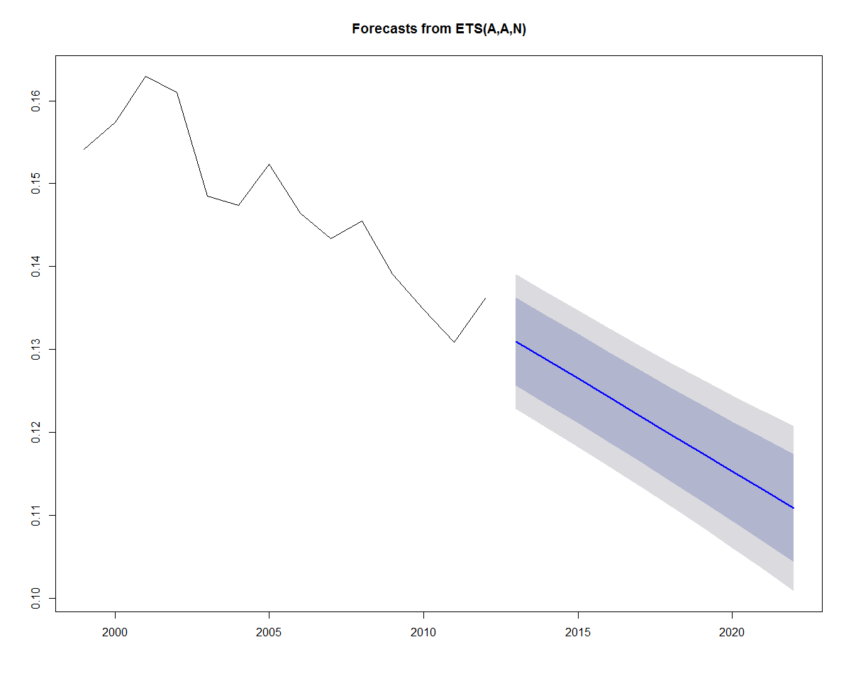

Earlier, we added a linear trend line to the data. If we wanted to incorporate a linear trend into the forecast as well, we can substitute A for the second parameter (trend parameter), which yields an "AAN" model (Holt's linear trend). This type of method allows exponential smoothing with a trend:
fit <- ets(x, model = "AAN")
summary(fit)
> ETS(A,A,N)
>
> Call:
> ets(y = x, model = "AAN")
>
> Smoothing parameters:
> alpha = 0.0312
> beta = 0.0312
>
> Initial states:
> l = 0.1641
> b = -0.0021
>
> sigma: 0.0042
>
> AIC AICc BIC
> -108.5711 -104.1267 -106.0149
>
> Training set error measures:
> ME RMSE MAE MPE MAPE
> Training set -0.000290753 0.004157744 0.003574276 -0.2632899 2.40212
> MASE ACF1
> Training set 0.7709083 0.05003007
Plotting the forecast yields the plot below:
plot(forecast(fit))