
Deep learning is a subcategory of machine learning inspired by the structure and functioning of a human brain. In recent times, deep learning has gained a lot of traction primarily because of higher computational power, bigger datasets, and better algorithms with (artificial) intelligent learning abilities and more inquisitiveness for data-driven insights. Before we get into the details of deep learning, let's understand some basic concepts of machine learning that form the basis for most analytical solutions.
Machine learning is an arena of developing algorithms with the ability to mine natural patterns from the data such that better decisions are made using predictive insights. These insights are pertinent across a horizon of real-world applications, from medical diagnosis (using computational biology) to real-time stock trading (using computational finance), from weather forecasting to natural language processing, from predictive maintenance (in automation and manufacturing) to prescriptive recommendations (in e-commerce and e-retail), and so on.
The following figure elucidates two primary techniques of machine learning; namely, supervised learning and unsupervised learning:
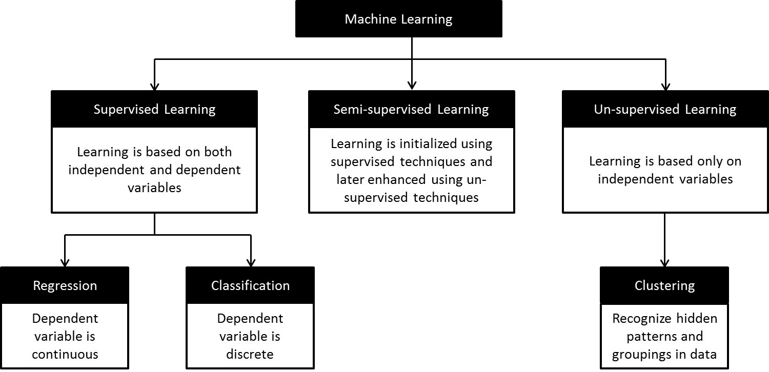
Classification of different techniques in machine learning
Supervised learning: Supervised learning is a form of evidence-based learning. The evidence is the known outcome for a given input and is in turn used to train the predictive model. Models are further classified into regression and classification, based on the outcome data type. In the former, the outcome is continuous, and in the latter the outcome is discrete. Stock trading and weather forecasting are some widely used applications of regression models, and span detection, speech recognition, and image classification are some widely used applications of classification models.
Some algorithms for regression are linear regression, Generalized Linear Models (GLM), Support Vector Regression (SVR), neural networks, decision trees, and so on; in classification, we have logistic regression, Support Vector Machines (SVM), Linear discriminant analysis (LDA), Naive Bayes, nearest neighbors, and so on.
Semi-supervised learning: Semi-supervised learning is a class of supervised learning using unsupervised techniques. This technique is very useful in scenarios where the cost of labeling an entire dataset is highly impractical against the cost of acquiring and analyzing unlabeled data.
Unsupervised learning: As the name suggests, learning from data with no outcome (or supervision) is called unsupervised learning. It is a form of inferential learning based on hidden patterns and intrinsic groups in the given data. Its applications include market pattern recognition, genetic clustering, and so on.
Some widely used clustering algorithms are k-means, hierarchical, k-medoids, Fuzzy C-means, hidden markov, neural networks, and many more.
Let's take a look at linear regression in supervised learning:
- Let's begin with a simple example of linear regression where we need to determine the relationship between men's height (in cms) and weight (in kgs). The following sample data represents the height and weight of 10 random men:
data <- data.frame("height" = c(131, 154, 120, 166, 108, 115,
158, 144, 131, 112),
"weight" = c(54, 70, 47, 79, 36, 48, 65,
63, 54, 40))- Now, generate a linear regression model as follows:
lm_model <- lm(weight ~ height, data)
- The following plot shows the relationship between men's height and weight along with the fitted line:
plot(data, col = "red", main = "Relationship between height and
weight",cex = 1.7, pch = 1, xlab = "Height in cms", ylab = "Weight
in kgs")
abline(lm(weight ~ height, data))
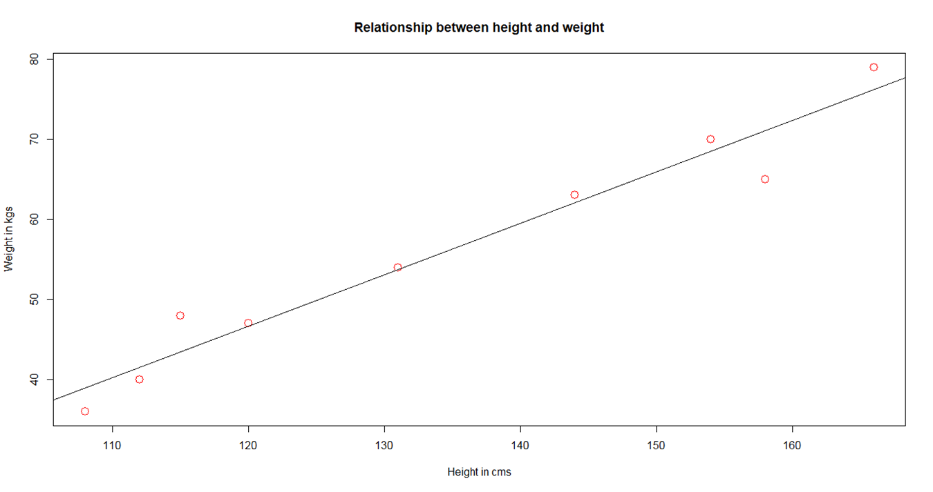
Linear relationship between weight and height
- In semi-supervised models, the learning is primarily initiated using labeled data (a smaller quantity in general) and then augmented using unlabeled data (a larger quantity in general).
Let's perform K-means clustering (unsupervised learning) on a widely used dataset, iris.
- This dataset consists of three different species of iris (Setosa, Versicolor, and Virginica) along with their distinct features such as sepal length, sepal width, petal length, and petal width:
data(iris)
head(iris)
Sepal.Length Sepal.Width Petal.Length Petal.Width Species
1 5.1 3.5 1.4 0.2 setosa
2 4.9 3.0 1.4 0.2 setosa
3 4.7 3.2 1.3 0.2 setosa
4 4.6 3.1 1.5 0.2 setosa
5 5.0 3.6 1.4 0.2 setosa
6 5.4 3.9 1.7 0.4 setosa
- The following plots show the variation of features across irises. Petal features show a distinct variation as against sepal features:
library(ggplot2)
library(gridExtra)
plot1 <- ggplot(iris, aes(Sepal.Length, Sepal.Width, color =
Species))
  geom_point(size = 2)
  ggtitle("Variation by Sepal features")
plot2 <- ggplot(iris, aes(Petal.Length, Petal.Width, color =
  Species))
   geom_point(size = 2)
   ggtitle("Variation by Petal features")
grid.arrange(plot1, plot2, ncol=2)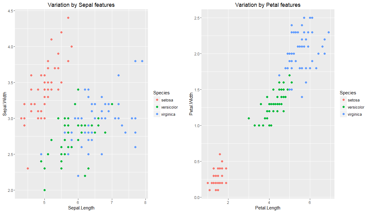
Variation of sepal and petal features by length and width
- As petal features show a good variation across irises, let's perform K-means clustering using the petal length and petal width:
set.seed(1234567)
iris.cluster <- kmeans(iris[, c("Petal.Length","Petal.Width")],
 3, nstart = 10)
iris.cluster$cluster <- as.factor(iris.cluster$cluster)- The following code snippet shows a cross-tab between clusters and species (irises). We can see that cluster 1 is primarily attributed with setosa, cluster 2 with versicolor, and cluster 3 with virginica:
> table(cluster=iris.cluster$cluster,species= iris$Species)
species
cluster setosa versicolor virginica
1 50 0 0
2 0 48 4
3 0 2 46

ggplot(iris, aes(Petal.Length, Petal.Width, color =
iris.cluster$cluster)) + geom_point() + ggtitle("Variation by
Clusters")
- The following plot shows the distribution of clusters:
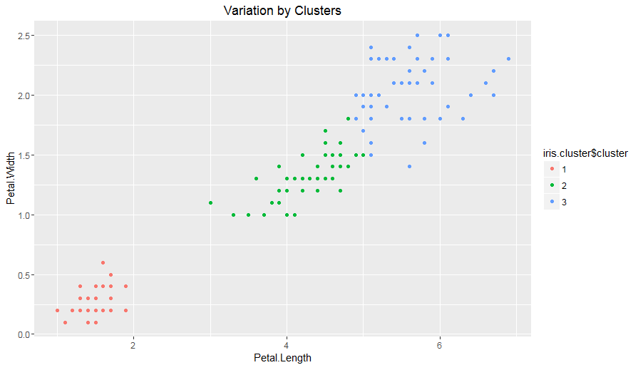
Variation of irises across three clusters
Model evaluation is a key step in any machine learning process. It is different for supervised and unsupervised models. In supervised models, predictions play a major role; whereas in unsupervised models, homogeneity within clusters and heterogeneity across clusters play a major role.
Some widely used model evaluation parameters for regression models (including cross validation) are as follows:
- Coefficient of determination
- Root mean squared error
- Mean absolute error
- Akaike or Bayesian information criterion
Some widely used model evaluation parameters for classification models (including cross validation) are as follows:
- Confusion matrix (accuracy, precision, recall, and F1-score)
- Gain or lift charts
- Area under ROC (receiver operating characteristic) curve
- Concordant and discordant ratio
Some of the widely used evaluation parameters of unsupervised models (clustering) are as follows:
- Contingency tables
- Sum of squared errors between clustering objects and cluster centers or centroids
- Silhouette value
- Rand index
- Matching index
- Pairwise and adjusted pairwise precision and recall (primarily used in NLP)
Bias and variance are two key error components of any supervised model; their trade-off plays a vital role in model tuning and selection. Bias is due to incorrect assumptions made by a predictive model while learning outcomes, whereas variance is due to model rigidity toward the training dataset. In other words, higher bias leads to underfitting and higher variance leads to overfitting of models.
In bias, the assumptions are on target functional forms. Hence, this is dominant in parametric models such as linear regression, logistic regression, and linear discriminant analysis as their outcomes are a functional form of input variables.
Variance, on the other hand, shows how susceptible models are to change in datasets. Generally, target functional forms control variance. Hence, this is dominant in non-parametric models such as decision trees, support vector machines, and K-nearest neighbors as their outcomes are not directly a functional form of input variables. In other words, the hyperparameters of non-parametric models can lead to overfitting of predictive models.