
We will demonstrate the main operations for data manipulation using pandas. This approach is used as a standard for other data manipulation tools, such as Spark, so it's helpful to learn how to manipulate data using pandas. It's common in a big data pipeline to convert part of the data or a data sample to a pandas DataFrame to apply a more complex transformation, to visualize the data, or to use more refined machine learning models with the scikit-learn library. Pandas is also fast for in-memory, single-machine operations. Although there is a memory overhead between the data size and the pandas DataFrame, it can be used to manipulate large volumes of data quickly.
We will learn how to apply the basic operations:
Read data into a DataFrame
Selection and filtering
Apply a function to data
GroupBy and aggregation
Visualize data from DataFrames
Let's start by reading data into a pandas DataFrame.
Pandas accepts several data formats and ways to ingest data. Let's start with the more common way, reading a CSV file. Pandas has a function called read_csv, which can be used to read a CSV file, either locally or from a URL. Let's read some data from the Socrata Open Data initiative, a RadNet Laboratory Analysis from the U.S. Environmental Protection Agency (EPA), which lists the radioactive content collected by the EPA.
How can an analyst start data analysis without data? We need to learn how to get data from an internet source into our notebook so that we can start our analysis. Let's demonstrate how pandas can read CSV data from an internet source so we can analyze it:
Import pandas library.
import pandas as pd
Read the Automobile mileage dataset, available at this URL: https://github.com/TrainingByPackt/Big-Data-Analysis-with-Python/blob/master/Lesson01/imports-85.data. Convert it to csv.
Use the column names to name the data, with the parameter names on the read_csv function.
Sample code : df = pd.read_csv("/path/to/imports-85.csv", names = columns)Use the function read_csv from pandas and show the first rows calling the method head on the DataFrame:
import pandas as pd
df = pd.read_csv("imports-85.csv")
df.head()
The output is as follows:

Figure 1.5: Entries of the Automobile mileage dataset
Pandas can read more formats:
JSON
Excel
HTML
HDF5
Parquet (with PyArrow)
SQL databases
Google Big Query
Try to read other formats from pandas, such as Excel sheets.
By data manipulation we mean any selection, transformation, or aggregation that is applied over the data. Data manipulation can be done for several reasons:
To select a subset of data for analysis
To clean a dataset, removing invalid, erroneous, or missing values
To group data into meaningful sets and apply aggregation functions
Pandas was designed to let the analyst do these transformations in an efficient way.
Pandas DataFrames can be sliced similarly to Python lists. For example, to select a subset of the first 10 rows of the DataFrame, we can use the [0:10] notation. We can see in the following screenshot that the selection of the interval [1:3] that in the NumPy representation selects the rows 1 and 2.
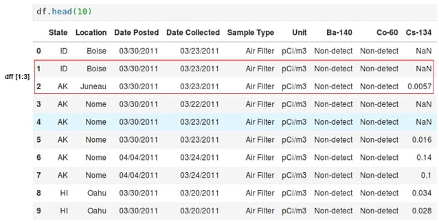
Figure 1.6: Selection in a pandas DataFrame
In the following section, we'll explore the selection and filtering operation in depth.
When performing data analysis, we usually want to see how data behaves differently under certain conditions, such as comparing a few columns, selecting only a few columns to help read the data, or even plotting. We may want to check specific values, such as the behavior of the rest of the data when one column has a specific value.
After selecting with slicing, we can use other methods, such as the head method, to select only a few rows from the beginning of the DataFrame. But how can we select some columns in a DataFrame?
To select a column, just use the name of the column. We will use the notebook. Let's select the cylinders column in our DataFrame using the following command:
df['State']
The output is as follows:
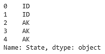
Figure 1.7: DataFrame showing the state
Another form of selection that can be done is filtering by a specific value in a column. For example, let's say that we want to select all rows that have the State column with the MN value. How can we do that? Try to use the Python equality operator and the DataFrame selection operation:
df[df.State == "MN"]
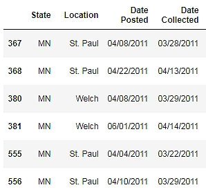
Figure 1.8: DataFrame showing the MN states
More than one filter can be applied at the same time. The OR, NOT, and AND logic operations can be used when combining more than one filter. For example, to select all rows that have State equal to AK and a Location of Nome, use the & operator:
df[(df.State == "AK") & (df.Location == "Nome")]
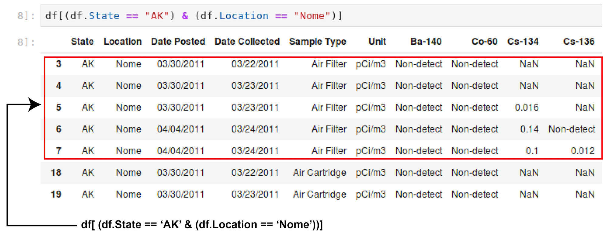
Figure 1.9: DataFrame showing State AK and Location Nome
Another powerful method is .loc. This method has two arguments, the row selection and the column selection, enabling fine-grained selection. An important caveat at this point is that, depending on the applied operation, the return type can be either a DataFrame or a series. The .loc method returns a series, as selecting only a column. This is expected, because each DataFrame column is a series. This is also important when more than one column should be selected. To do that, use two brackets instead of one, and use as many columns as you want to select.
As we saw before, selecting data, separating variables, and viewing columns and rows of interest is fundamental to the analysis process. Let's say we want to analyze the radiation from I-131 in the state of Minnesota:
Import the NumPy and pandas libraries using the following command in the Jupyter notebook:
import numpy as np
import pandas as pd
Read the RadNet dataset from the EPA, available from the Socrata project at https://github.com/TrainingByPackt/Big-Data-Analysis-with-Python/blob/master/Lesson01/RadNet_Laboratory_Analysis.csv:
url = "https://opendata.socrata.com/api/views/cf4r-dfwe/rows.csv?accessType=DOWNLOAD"
df = pd.read_csv(url)
Start by selecting a column using the ['<name of the column>'] notation. Use the State column:
df['State'].head()
The output is as follows:
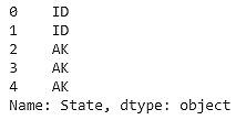
Figure 1.10: Data in the State column
Now filter the selected values in a column using the MN column name:
df[df.State == "MN"]
The output is as follows:
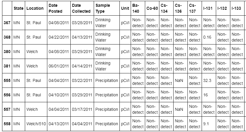
Figure 1.11: DataFrame showing States with MN
Select more than one column per condition. Add the Sample Type column for filtering:
df[(df.State == 'CA') & (df['Sample Type'] == 'Drinking Water')]
The output is as follows:
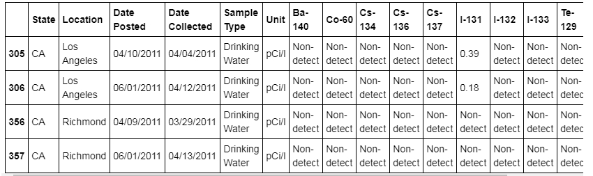
Figure 1.12: DataFrame with State CA and Sample type as Drinking water
Next, select the MN state and the isotope I-131:
df[(df.State == "MN") ]["I-131"]
The output is as follows:
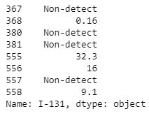
Figure 1.13: Data showing the DataFrame with State Minnesota and Isotope I-131
The radiation in the state of Minnesota with ID 555 is the highest.
We can do the same more easily with the .loc method, filtering by state and selecting a column on the same .loc call:
df_rad.loc[df_rad.State == "MN", "I-131"]
df[['I-132']].head()
The output is as follows:
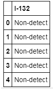
Figure 1.14: DataFrame with I-132
In this exercise, we learned how to filter and select values, either on columns or rows, using the NumPy slice notation or the .loc method. This can help when analyzing data, as we can check and manipulate only a subset of the data instead having to handle the entire dataset at the same time.
Note
The result of the .loc filter is a series and not a DataFrame. This depends on the operation and selection done on the DataFrame and not is caused only by .loc. Because the DataFrame can be understood as a 2D combination of series, the selection of one column will return a series. To make a selection and still return a DataFrame, use double brackets:
df[['I-132']].head()
Data is never clean. There are always cleaning tasks that have to be done before a dataset can be analyzed. One of the most common tasks in data cleaning is applying a function to a column, changing a value to a more adequate one. In our example dataset, when no concentration was measured, the non-detect value was inserted. As this column is a numerical one, analyzing it could become complicated. We can apply a transformation over a column, changing from non-detect to numpy.NaN, which makes manipulating numerical values more easy, filling with other values such as the mean, and so on.
To apply a function to more than one column, use the applymap method, with the same logic as the apply method. For example, another common operation is removing spaces from strings. Again, we can use the apply and applymap functions to fix the data. We can also apply a function to rows instead of to columns, using the axis parameter (0 for rows, 1 for columns).
Before starting an analysis, we need to check for data problems, and when we find them (which is very common!), we have to correct the issues by transforming the DataFrame. One way to do that, for instance, is by applying a function to a column, or to the entire DataFrame. It's common for some numbers in a DataFrame, when it's read, to not be converted correctly to floating-point numbers. Let's fix this issue by applying functions:
Import pandas and numpy library.
Read the RadNet dataset from the U.S. Environmental Protection Agency.
Create a list with numeric columns for radionuclides in the RadNet dataset.
Use the apply method on one column, with a lambda function that compares the Non-detect string.
Replace the text values by NaN in one column with np.nan.
Use the same lambda comparison and use the applymap method on several columns at the same time, using the list created in the first step.
Create a list of the remaining columns that are not numeric.
Remove any spaces from these columns.
Using the selection and filtering methods, verify that the names of the string columns don't have any more spaces.
The spaces in column names can be extraneous and can make selection and filtering more complicated. Fixing the numeric types helps when statistics must be computed using the data. If there is a value that is not valid for a numeric column, such as a string in a numeric column, the statistical operations will not work. This scenario happens, for example, when there is an error in the data input process, where the operator types the information by hand and makes mistakes, or the storage file was converted from one format to another, leaving incorrect values in the columns.