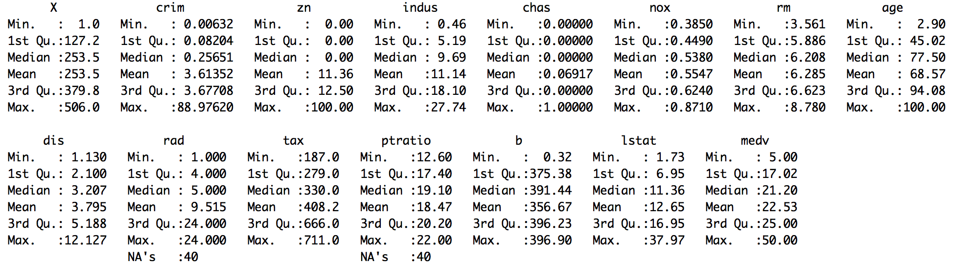
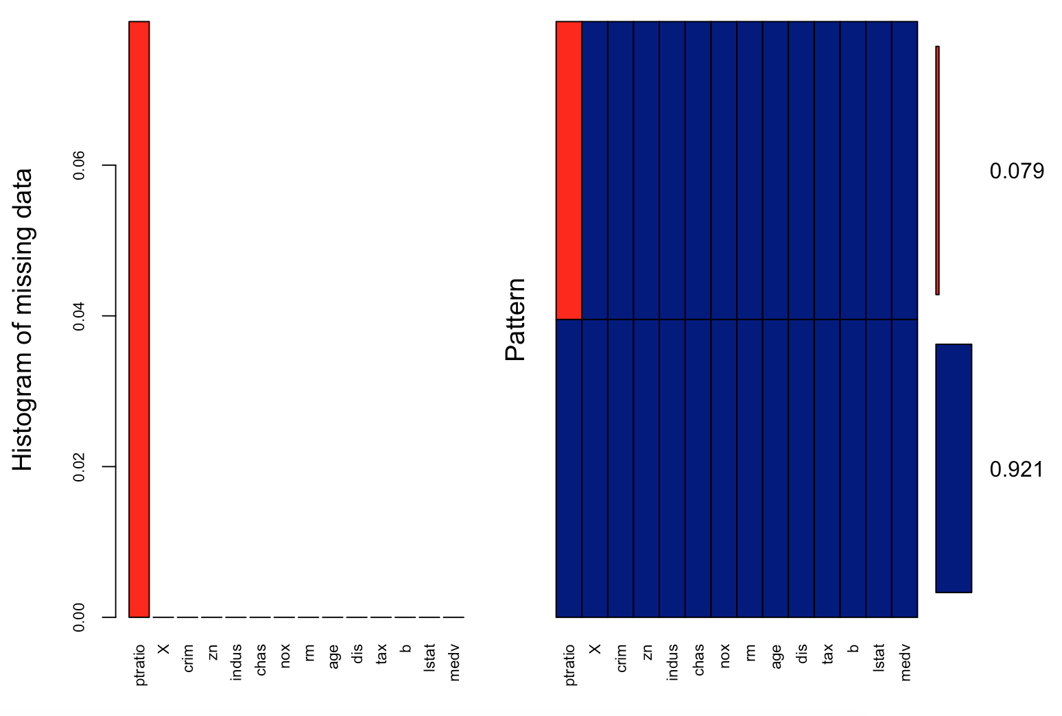
In most real-world problems, data is likely to be incomplete because of incorrect data entry, faulty equipment, or improperly coded data. In R, missing values are represented by the symbol NA (not available) and are considered to be the first obstacle in predictive modeling. So, it's always a good idea to check for missing data in a dataset before proceeding for further predictive analysis. This recipe shows you how to handle missing data.

R provides three simple ways to handle missing values:

1. Deleting the observations.
2. Deleting the variables.
3. Replacing the values with mean, median, or mode.

Install the package in your R environment as follows:

> install.packages("Hmisc")

If you have not already downloaded the files for this chapter, do it now and ensure that the housing-with-missing-value.csv file is in your R working directory.

Once the files are ready, load the Hmisc package and read the files as follows:

1. Load the CSV data from the files:

> housing.dat <- read.csv("housing-with-missing-value.csv",header = TRUE, stringsAsFactors = FALSE)

2. Check summary of the dataset:

> summary(housing.dat)            

The output would be as follows:

3. Delete the missing observations from the dataset, removing all NAs with list-wise deletion:

> housing.dat.1 <- na.omit(housing.dat)

Remove NAs from certain columns:

> drop_na <- c("rad")
> housing.dat.2 <-housing.dat [complete.cases(housing.dat [ , !(names(housing.dat)) %in% drop_na]),]

4. Finally, verify the dataset with summary statistics:

> summary(housing.dat.1$rad)
 Min. 1st Qu. Median Mean 3rd Qu. Max.
 1.000 4.000 5.000 9.599 24.000 24.000

> summary(housing.dat.1$ptratio)
 Min. 1st Qu. Median Mean 3rd Qu. Max.
 12.60 17.40 19.10 18.47 20.20 22.00

> summary(housing.dat.2$rad)
 Min. 1st Qu. Median Mean 3rd Qu. Max. NA's
 1.000 4.000 5.000 9.599 24.000 24.000 35

> summary(housing.dat.2$ptratio)
 Min. 1st Qu. Median Mean 3rd Qu. Max.
 12.60 17.40 19.10 18.47 20.20 22.00

5. Delete the variables that have the most missing observations:

# Deleting a single column containing many NAs
> housing.dat.3 <- housing.dat$rad <- NULL

#Deleting multiple columns containing NAs:
> drops <- c("ptratio","rad")
>housing.dat.4 <- housing.dat[ , !(names(housing.dat) %in% drops)]

Finally, verify the dataset with summary statistics:

> summary(housing.dat.4)

6. Load the library:

> library(Hmisc)

7. Replace the missing values with mean, median, or mode:

#replace with mean
> housing.dat$ptratio <- impute(housing.dat$ptratio, mean)
> housing.dat$rad <- impute(housing.dat$rad, mean)

#replace with median
> housing.dat$ptratio <- impute(housing.dat$ptratio, median)
> housing.dat$rad <- impute(housing.dat$rad, median) 

#replace with mode/constant value
> housing.dat$ptratio <- impute(housing.dat$ptratio, 18)
> housing.dat$rad <- impute(housing.dat$rad, 6)

Finally, verify the dataset with summary statistics:

> summary(housing.dat)

When you have large numbers of observations in your dataset and all the classes to be predicted are sufficiently represented by the data points, then deleting missing observations would not introduce bias or disproportionality of output classes.

In the housing.dat dataset, we saw from the summary statistics that the dataset has two columns, ptratio and rad, with missing values.

The na.omit() function lets you remove all the missing values from all the columns of your dataset, whereas the complete.cases() function lets you remove the missing values from some particular column/columns.

Sometimes, particular variable/variables might have more missing values than the rest of the variables in the dataset. Then it is better to remove that variable unless it is a really important predictor that makes a lot of business sense. Assigning NULL to a variable is an easy way of removing it from the dataset.

In both, the given way of handling missing values through the deletion approach reduces the total number of observations (or rows) from the dataset. Instead of removing missing observations or removing a variable with many missing values, replacing the missing values with the mean, median, or mode is often a crude way of treating the missing values. Depending on the context, such as if the variation is low or if the variable has low leverage over the response/target, such a naive approximation is acceptable and could possibly give satisfactory results. The impute() function in the Hmisc library provides an easy way to replace the missing value with the mean, median, or mode (constant).

Sometime it is better to understand the missing pattern in the dataset through visualization before taking further decision about elimination or imputation of the missing values.

Let us use the md.pattern() function from the mice package to get a better understanding of the pattern of missing data.

> library(mice)
> md.pattern(housing.dat)

We can notice from the output above that 466 samples are complete, 40 samples miss only the ptratio value.

Next we will visualize the housing data to understand missing information using aggr_plot method from VIM package:

> library(VIM)
> aggr_plot <- aggr(housing.dat, col=c('blue','red'), numbers=TRUE, sortVars=TRUE, labels=names(housing.dat), cex.axis=.7, gap=3, ylab=c("Histogram of missing data","Pattern"))

We can understand from the plot that almost 92.1% of the samples are complete and only 7.9% are missing information from the ptratio values.