TensorFlow is very unlike other programming languages. We first need to build a blueprint of whatever neural network we want to create. This is accomplished by dividing the program into two separate parts, namely, definition of the computational graph and its execution. At first, this might appear cumbersome to the conventional programmer, but it is this separation of the execution graph from the graph definition that gives TensorFlow its strength, that is, the ability to work on multiple platforms and parallel execution.

Computational graph: A computational graph is a network of nodes and edges. In this section, all the data to be used, in other words, tensor Objects (constants, variables, and placeholders) and all the computations to be performed, namely, Operation Objects (in short referred as ops), are defined. Each node can have zero or more inputs but only one output. Nodes in the network represent Objects (tensors and Operations), and edges represent the Tensors that flow between operations. The computation graph defines the blueprint of the neural network but Tensors in it have no value associated with them yet.

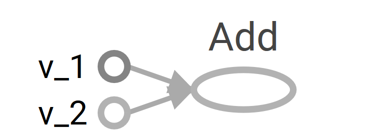
To build a computation graph we define all the constants, variables, and operations that we need to perform. Constants, variables, and placeholders will be dealt with in the next recipe. Mathematical operations will be dealt in detail in the recipe for matrix manipulations. Here, we describe the structure using a simple example of defining and executing a graph to add two vectors.

Execution of the graph: The execution of the graph is performed using Session Object. The Session Object encapsulates the environment in which tensor and Operation Objects are evaluated. This is the place where actual calculations and transfer of information from one layer to another takes place. The values of different tensor Objects are initialized, accessed, and saved in Session Object only. Up to now the tensor Objects were just abstract definitions, here they come to life.

We proceed with the recipe as follows:

1. We consider a simple example of adding two vectors, we have two inputs vectors v_1 and v_2 they are to be fed as input to the Add operation. The graph we want to build is as follows:

2. The corresponding code to define the computation graph is as follows:

v_1 = tf.constant([1,2,3,4]) 
v_2 = tf.constant([2,1,5,3]) 
v_add = tf.add(v_1,v_2)  # You can also write v_1 + v_2 instead 

3. Next, we execute the graph in the session:

with tf.Session() as sess: 
    prin(sess.run(v_add)) 

The above two commands are equivalent to the following code. The advantage of using with block is that one need not close the session explicitly.

sess = tf.Session() 
print(ses.run(tv_add)) 
sess.close() 

4. This results in printing the sum of two vectors:

[3 3 8 7] 

The building of a computational graph is very simple; you go on adding the variables and operations and passing them through (flow the tensors) in the sequence you build your neural network layer by layer. TensorFlow also allows you to use specific devices (CPU/GPU) with different objects of the computation graph using with tf.device(). In our example, the computational graph consists of three nodes, v_1 and v_2 representing the two vectors, and Add is the operation to be performed on them.

Now, to bring this graph to life, we first need to define a session object using tf.Session(); we gave the name sess to our session object. Next, we run it using the run method defined in Session class as follows:

run (fetches, feed_dict=None, options=None, run_metadata) 

This evaluates the tensor in fetches; our example has tensor v_add in fetches. The run method will execute every tensor and every operation in the graph leading to v_add. If instead of v_add, you have v_1 in fetches, the result will be the value of vector v_1:

[1,2,3,4]  

Fetches can be a single tensor/operation object or more, for example, if the fetches is [v_1, v_2, v_add], the output will be the following:

[array([1, 2, 3, 4]), array([2, 1, 5, 3]), array([3, 3, 8, 7])] 

In the same program code, we can have many session objects.

You must be wondering why we have to write so many lines of code for a simple vector addition or to print a small message. Well, you could have very conveniently done this work in a one-liner:

print(tf.Session().run(tf.add(tf.constant([1,2,3,4]),tf.constant([2,1,5,3])))) 

Writing this type of code not only affects the computational graph but can be memory expensive when the same operation ( OP) is performed repeatedly in a for loop. Making a habit of explicitly defining all tensor and operation objects not only makes the code more readable but also helps you visualize the computational graph in a cleaner manner.

If you are working on Jupyter Notebook or Python shell, it is more convenient to use tf.InteractiveSession instead of tf.Session. InteractiveSession makes itself the default session so that you can directly call run the tensor Object using eval() without explicitly calling the session, as described in the following example code:

sess = tf.InteractiveSession() 
 
v_1 = tf.constant([1,2,3,4]) 
v_2 = tf.constant([2,1,5,3]) 
 
v_add = tf.add(v_1,v_2) 
 
print(v_add.eval()) 
 
sess.close()