Book Image

Neural Network Projects with Python

By : James Loy
Book Image

Neural Network Projects with Python

By: James Loy

Overview of this book

Neural networks are at the core of recent AI advances, providing some of the best resolutions to many real-world problems, including image recognition, medical diagnosis, text analysis, and more. This book goes through some basic neural network and deep learning concepts, as well as some popular libraries in Python for implementing them. It contains practical demonstrations of neural networks in domains such as fare prediction, image classification, sentiment analysis, and more. In each case, the book provides a problem statement, the specific neural network architecture required to tackle that problem, the reasoning behind the algorithm used, and the associated Python code to implement the solution from scratch. In the process, you will gain hands-on experience with using popular Python libraries such as Keras to build and train your own neural networks from scratch. By the end of this book, you will have mastered the different neural network architectures and created cutting-edge AI projects in Python that will immediately strengthen your machine learning portfolio.
Table of Contents (10 chapters)

Neural networks

Neural networks are a class of machine learning algorithms that are loosely inspired by neurons in the human brain. However, without delving too much into brain analogies, I find it easier to simply describe neural networks as a mathematical function that maps a given input to the desired output. To understand what that means, let's take a look at a single layer neural network (known as a perceptron).

A Perceptron can be illustrated with the following diagram:

At its core, the Perceptron is simply a mathematical function that takes in a set of inputs, performs some mathematical computation, and outputs the result of the computation. In this case, that mathematical function is simply this:

refers to the weights of the Perceptron. We will explain what the weights in a neural network refers to in the next few sections. For now, we just need to keep in mind that neural networks are simply mathematical functions that map a given input to a desired output.

Why neural networks?

Before we dive into creating our own neural network, it is worth understanding why neural networks have gained such an important foothold in machine learning and AI.

The first reason is that neural networks are universal function approximators. What that means is that given any arbitrary function that we are trying to model, no matter how complex, neural networks are always able to represent that function. This has a profound implication on neural networks and AI in general. Assuming that any problem in the world can be described by a mathematical function (no matter how complex), we can use neural networks to represent that function, effectively modeling anything in the world. A caveat to this is that while scientists have proved the universality of neural networks, a large and complex neural network may never be trained and generalized correctly.

The second reason is that the architecture of neural networks are highly scalable and flexible. As we will see in the next section, we can easily stack layers in each neural network, increasing the complexity of the neural network. Perhaps more interestingly, the capabilities of neural networks are only limited by our own imagination. Through creative neural network architecture design, machine learning engineers have learned how to use neural networks to predict time series data (known as recurrent neural networks (RNNs)), which are used in areas such as speech recognition. In recent years, scientists have also shown that by pitting two neural networks against each other in a contest (known as a generative adversarial network (GAN)), we can generate photorealistic images that are indistinguishable to the human eye.

The basic architecture of neural networks

In this section, we will look at the basic architecture of neural networks, the building blocks on which all complex neural networks are based. We will also code up our own basic neural network from scratch in Python, without any machine learning libraries. This exercise will help you gain an intuitive understanding of the inner workings of neural networks.

Neural networks consist of the following components:

  • An input layer, x
  • An arbitrary amount of hidden layers
  • An output layer, ŷ
  • A set of weights and biases between each layer, W and b
  • A choice of activation function for each hidden layer, σ

The following diagram shows the architecture of a two-layer neural network (note that the input layer is typically excluded when counting the number of layers in a neural network):

Training a neural network from scratch in Python

Now that we understand the basic architecture of a neural network, let's create our own neural network from scratch in Python.

First, let's create a NeuralNetwork class in Python:

import numpy as np

class NeuralNetwork:
def __init__(self, x, y):
self.input = x
self.weights1 = np.random.rand(self.input.shape[1],4)
self.weights2 = np.random.rand(4,1)
self.y = y
self.output = np.zeros(self.y.shape)
Notice that in the preceding code, we initialize the weights (self.weights1 and self.weights2) as a NumPy array with random values. NumPy arrays are used to represent multidimensional arrays in Python. The exact dimensions of our weights are specified in the parameters of the np.random.rand() function. For the dimensions of the first weight array, we use a variable (self.input.shape[1]) to create an array of variable dimensions, depending on the size of our input.

The output, ŷ, of a simple two-layer neural network is as follows:

You might notice that in the preceding equation, the weights, W, and the biases, b, are the only variables that affects the output, ŷ.

Naturally, the right values for the weights and biases determine the strength of the predictions. The process of fine-tuning the weights and biases from the input data is known as training the neural network.

Each iteration of the training process consists of the following steps:

  1. Calculating the predicted output ŷ, known as Feedforward
  2. Updating the weights and biases, known as Backpropagation

The following sequential graph illustrates the process:

Feedforward

As we've seen in the preceding sequential graph, feedforward is just simple calculus, and for a basic two-layer neural network, the output of the neural network is as follows:

Let's add a feedforward function in our Python code to do exactly that. Note that for simplicity, we have assumed the biases to be 0:

import numpy as np

def sigmoid(x):
return 1.0/(1 + np.exp(-x))

class NeuralNetwork:
def __init__(self, x, y):
self.input = x
self.weights1 = np.random.rand(self.input.shape[1],4)
self.weights2 = np.random.rand(4,1)
self.y = y
self.output = np.zeros(self.y.shape)

def feedforward(self):
self.layer1 = sigmoid(np.dot(self.input, self.weights1))
self.output = sigmoid(np.dot(self.layer1, self.weights2))

However, we still need a way to evaluate the accuracy of our predictions (that is, how far off our predictions are). The loss function allows us to do exactly that.

The loss function

There are many available loss functions, and the nature of our problem should dictate our choice of loss function. For now, we'll use a simple Sum-of-Squares Error as our loss function:

The sum-of-squares error is simply the sum of the difference between each predicted value and the actual value. The difference is squared so that we measure the absolute value of the difference.

Our goal in training is to find the best set of weights and biases that minimizes the loss function.

Backpropagation

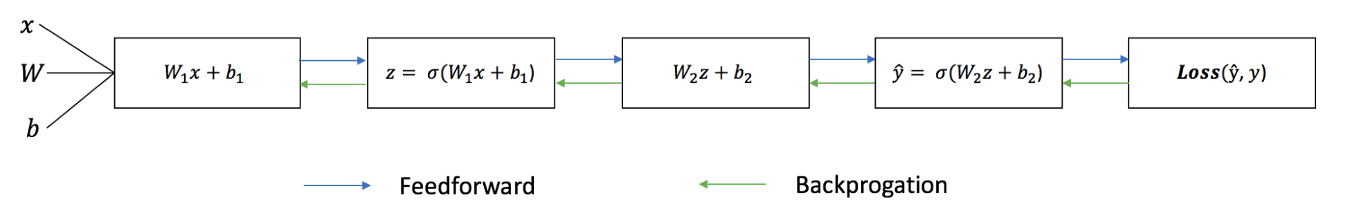
Now that we've measured the error of our prediction (loss), we need to find a way to propagate the error back, and to update our weights and biases.

In order to know the appropriate amount to adjust the weights and biases by, we need to know the derivative of the loss function with respect to the weights and biases.

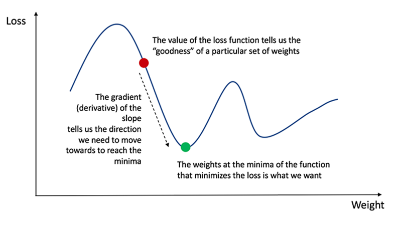
Recall from calculus that the derivative of a function is simply the slope of the function:

If we have the derivative, we can simply update the weights and biases by increasing/reducing with it (refer to the preceding diagram). This is known as gradient descent.

However, we can't directly calculate the derivative of the loss function with respect to the weights and biases because the equation of the loss function does not contain the weights and biases. We need the chain rule to help us calculate it. At this point, we are not going to delve into the chain rule because the math behind it can be rather complicated. Furthermore, machine learning libraries such as Keras takes care of gradient descent for us without requiring us to work out the chain rule from scratch. The key idea that we need to know is that once we have the derivative (slope) of the loss function with respect to the weights, we can adjust the weights accordingly.

Now let's add the backprop function into our Python code:

import numpy as np

def sigmoid(x):
return 1.0/(1 + np.exp(-x))

def sigmoid_derivative(x):
return x * (1.0 - x)

class NeuralNetwork:
def __init__(self, x, y):
self.input = x
self.weights1 = np.random.rand(self.input.shape[1],4)
self.weights2 = np.random.rand(4,1)
self.y = y
self.output = np.zeros(self.y.shape)

def feedforward(self):
self.layer1 = sigmoid(np.dot(self.input, self.weights1))
self.output = sigmoid(np.dot(self.layer1, self.weights2))

def backprop(self):
# application of the chain rule to find the derivation of the
# loss function with respect to weights2 and weights1
d_weights2 = np.dot(self.layer1.T, (2*(self.y - self.output) *
sigmoid_derivative(self.output)))
d_weights1 = np.dot(self.input.T, (np.dot(2*(self.y - self.output)
* sigmoid_derivative(self.output), self.weights2.T) *
sigmoid_derivative(self.layer1)))

self.weights1 += d_weights1
self.weights2 += d_weights2

if __name__ == "__main__":
X = np.array([[0,0,1],
[0,1,1],
[1,0,1],
[1,1,1]])
y = np.array([[0],[1],[1],[0]])
nn = NeuralNetwork(X,y)

for i in range(1500):
nn.feedforward()
nn.backprop()

print(nn.output)
Notice that in the preceding code, we used a sigmoid function in the feedforward function. The sigmoid function is an activation function to squash the values between 0 and 1. This is important because we need our predictions to be between 0 and 1 for this binary prediction problem. We will go through the sigmoid activation function in greater detail in the next chapter, Chapter 2, Predicting Diabetes with Multilayer Perceptrons.
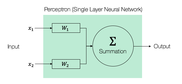
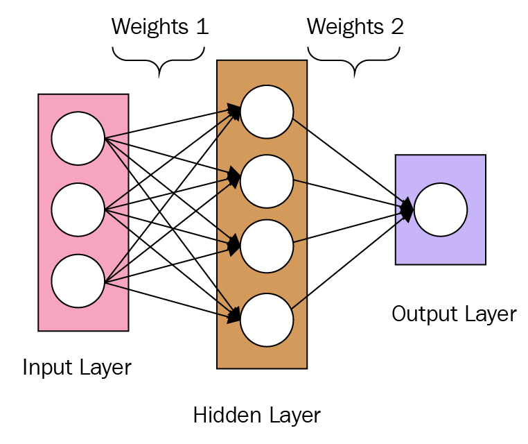
Putting it all together

Now that we have our complete Python code for doing feedforward and backpropagation, let's apply our neural network on an example and see how well it does.

The following table contains four data points, each with three input variables ( x1, x2, and x3) and a target variable (Y):

x1 x2 x3 Y
0 0 1 0
0 1 1 1
1 0 1 1
1 1 1 0

Our neural network should learn the ideal set of weights to represent this function. Note that it isn't exactly trivial for us to work out the weights just by inspection alone.

Let's train the neural network for 1,500 iterations and see what happens. Looking at the following loss-per-iteration graph, we can clearly see the loss monotonically decreasing toward a minimum. This is consistent with the gradient descent algorithm that we discussed earlier:

Let's look at the final prediction (output) from the neural network after 1,500 iterations:

Prediction Y (Actual)
0.023 0
0.979 1
0.975 1
0.025 0

We did it! Our feedforward and backpropagation algorithm trained the neural network successfully and the predictions converged on the true values.

Note that there's a slight difference between the predictions and the actual values. This is desirable, as it prevents overfitting and allows the neural network to generalize better to unseen data.

Now that we understand the inner workings of a neural network, we will introduce the machine learning libraries in Python that we will use for the rest of the book. Don't worry if you find it difficult to create your own neural network from scratch at this point. For the rest of the book, we'll be using libraries that will greatly simplify the process of building and training a neural network.

Deep learning and neural networks

What about deep learning? How is it different from neural networks? To put it simply, deep learning is a machine learning algorithm that uses multiple layers in a neural network for learning (also known as deep nets). While we can think of a single-layer perceptron as the simplest neural network, deep nets are simply neural networks on the opposite end of the complexity spectrum.

In a deep neural network (DNN), each layer learns information of increasing complexity, before passing it to successive layers. For example, when a DNN is trained for the purpose of facial recognition, the first few layers learn to identify edges in faces, followed by contours such as eyes and eventually complete facial features.

Although perceptrons were introduced back in the 1950s, deep learning did not take off until a few years ago. A key reason for the relatively slow progress of deep learning in the past few centuries is largely due to a lack of data and a lack of computation power. In the past few years, however, we have witnessed deep learning driving key innovations in machine learning and AI. Today, deep learning is the algorithm of choice when it comes to image recognition, autonomous vehicles, speech recognition, and game playing. So, what changed over the last few years?

In recent years, computer storage has become affordable enough to collect and store the massive amount of data that deep learning requires. It is becoming increasingly affordable to keep massive amount of data in the cloud, where it can be accessed by a cluster of computers from anywhere on earth. With the affordability of data storage, data is also becoming democratized. For example, websites such as ImageNet provides 14 million different images for deep learning researchers. Data is no longer a commodity that is owned by a privileged few.

The computational power that deep learning requires is also becoming more affordable and powerful. Most of deep learning today is powered by graphics processing units (GPUs), which excel in the computation required by DNNs. Keeping with the theme of democratization, many websites also provides free GPU processing power for deep learning enthusiasts. For example, Google Colab provides a free Tesla K80 GPU in the cloud for deep learning, available for anyone to use.

With these recent advancements, deep learning is becoming available to everyone. In the next few sections, we will introduce the Python libraries that we will use for deep learning.