Book Image

Neural Network Projects with Python

By : James Loy
Book Image

Neural Network Projects with Python

By: James Loy

Overview of this book

Neural networks are at the core of recent AI advances, providing some of the best resolutions to many real-world problems, including image recognition, medical diagnosis, text analysis, and more. This book goes through some basic neural network and deep learning concepts, as well as some popular libraries in Python for implementing them. It contains practical demonstrations of neural networks in domains such as fare prediction, image classification, sentiment analysis, and more. In each case, the book provides a problem statement, the specific neural network architecture required to tackle that problem, the reasoning behind the algorithm used, and the associated Python code to implement the solution from scratch. In the process, you will gain hands-on experience with using popular Python libraries such as Keras to build and train your own neural networks from scratch. By the end of this book, you will have mastered the different neural network architectures and created cutting-edge AI projects in Python that will immediately strengthen your machine learning portfolio.
Table of Contents (10 chapters)

pandas – a powerful data analysis toolkit in Python

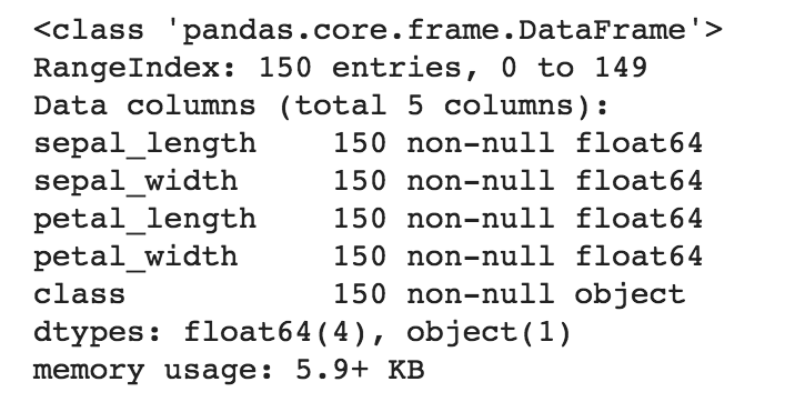
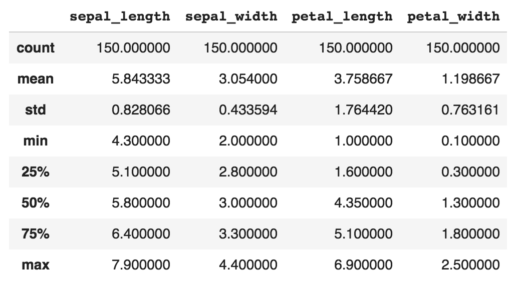
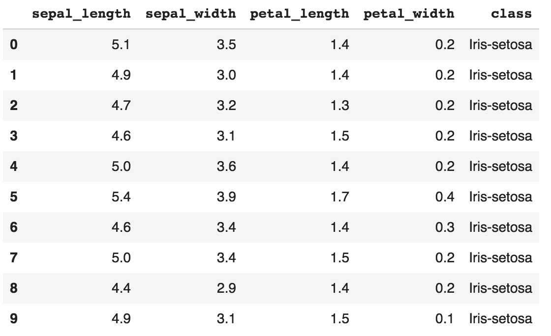
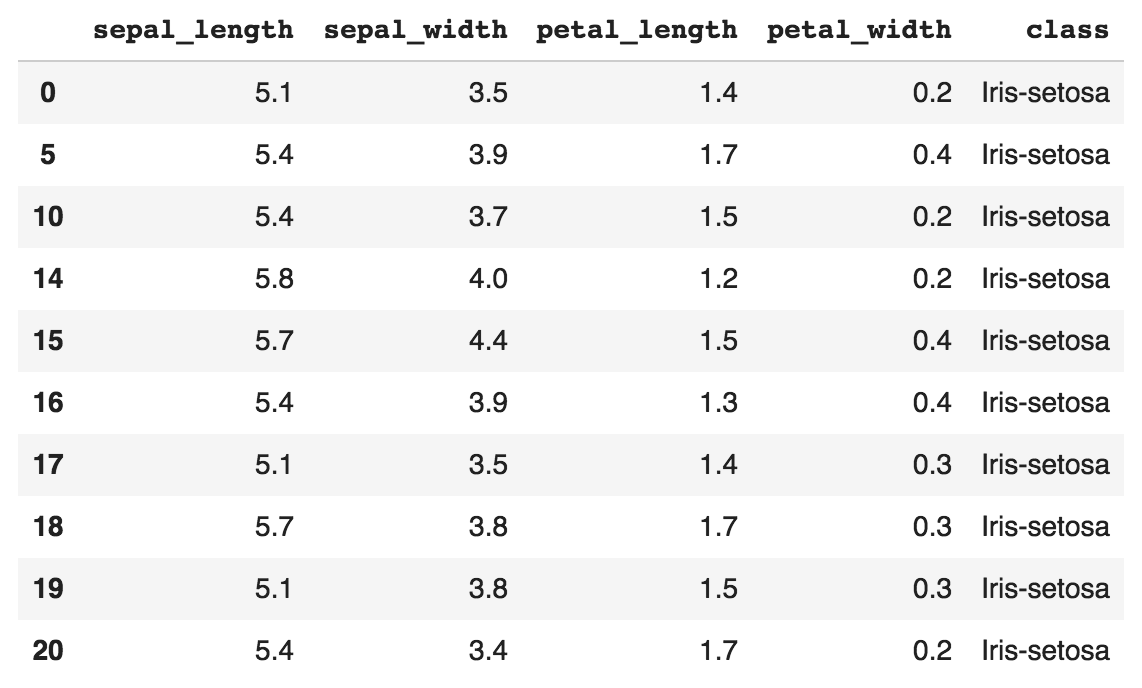
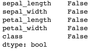
pandas is perhaps the most ubiquitous library in Python for data analysis. Built upon the powerful NumPy library, pandas provides a fast and flexible data structure in Python for handling real-world datasets. Raw data is often presented in tabular form, shared using the .csv file format. pandas provides a simple interface for importing these .csv files into a data structure known as DataFrames that makes it extremely easy to manipulate data in Python.

pandas DataFrames

pandas DataFrames are two-dimensional data structures, which you can think of as spreadsheets in Excel. DataFrames allow us to easily import the .csv files using a simple command. For example, the following sample code allows us to import the raw_data.csv file:

import pandas as pd
df = pd.read_csv("raw_data.csv")

Once the data is imported as a DataFrame, we can easily perform data preprocessing on it. Let's work through it using the Iris flower dataset. The Iris flower dataset is a commonly used dataset that contains data on the measurements (sepal length and width, petal length and width) of several classes of flowers. First, let's import the dataset as provided for free by University of California Irvine (UCI). Notice that pandas is able to import a dataset directly from a URL:

URL = \
'https://archive.ics.uci.edu/ml/machine-learning-databases/iris/iris.data'
df = pd.read_csv(URL, names = ['sepal_length', 'sepal_width',
'petal_length', 'petal_width', 'class'])

Now that it's in a DataFrame, we can easily manipulate the data. First, let's get a summary of the data as it is always important to know what kind of data we're working with:

print(df.info())

The output will be as shown in the following screenshot:

It looks like there are 150 rows in the dataset, with four numeric columns containing information regarding the sepal_length and sepal_width, along with the petal_length and petal_width. There is also one non-numeric column containing information regarding the class (that is, species) of the flowers.

We can get a quick statistical summary of the four numeric columns by calling the describe() function:

print(df.describe())

The output is shown in the following screenshot:

Next, let's take a look at the first 10 rows of the data:

print(df.head(10))

The output is shown in the following screenshot:

Simple, isn't it? pandas also allows us to perform data wrangling easily. For example, we can do the following to filter and select rows with sepal_length greater than 5.0:

df2 = df.loc[df['sepal_length'] > 5.0, ]

The output is shown in the following screenshot:

The loc command allows us to access a group of rows and columns.

Data visualization in pandas

EDA is perhaps one of the most important steps in the machine learning workflow, and pandas makes it extremely easy to visualize data in Python. pandas provides a high-level API for the popular matplotlib library, which makes it easy to construct plots directly from DataFrames.

As an example, let's visualize the Iris dataset using pandas to uncover important insights. Let's plot a scatterplot to visualize how sepal_width is related to sepal_length. We can construct a scatterplot easily using the DataFrame.plot.scatter() method, which is built into all DataFrames:

# Define marker shapes by class
import matplotlib.pyplot as plt
marker_shapes = ['.', '^', '*']

# Then, plot the scatterplot
ax = plt.axes()
for i, species in enumerate(df['class'].unique()):
species_data = df[df['class'] == species]
species_data.plot.scatter(x='sepal_length',
y='sepal_width',
marker=marker_shapes[i],
s=100,
title="Sepal Width vs Length by Species",
label=species, figsize=(10,7), ax=ax)

We'll get a scatterplot, as shown in the following screenshot:

From the scatterplot, we can notice some interesting insights. First, the relationship between sepal_width and sepal_length is dependent on the species. Setosa (dots) has a fairly linear relationship between sepal_width and sepal_length, while versicolor (triangle) and virginica (star) tends to have much greater sepal_length than Setosa. If we're designing a machine learning algorithm to predict the type of species of flower, we know that the sepal_width and sepal_length are important features to include in our model.

Next, let's plot a histogram to investigate the distribution. Consistent with scatterplots, pandas DataFrames provides a built in method to plot histograms using the DataFrame.plot.hist() function:

df['petal_length'].plot.hist(title='Histogram of Petal Length')

And we can see the output in the following screenshot:

We can see that the distribution of petal lengths is essentially bimodal. It appears that certain species of flowers have shorter petals than the rest. We can also plot a boxplot of the data. The boxplot is an important data visualization tool used by data scientists to understand the distribution of the data based on the first quartile, median, and the third quartile:

df.plot.box(title='Boxplot of Sepal Length & Width, and Petal Length & Width')

The output is given in the following screenshot:

From the boxplot, we can see that the variance of sepal_width is much smaller than the other numeric variables, with petal_length having the greatest variance.

We have now seen how convenient and easy it is to visualize data using pandas directly. Keep in mind that EDA is a crucial step in the machine learning pipeline, and it is something that we will continue to do in every project for the rest of the book.

Data preprocessing in pandas

Lastly, let's take a look at how we can use pandas for data preprocessing, specifically to encode categorical variables and to impute missing values.

Encoding categorical variables

In machine learning projects, it is common to receive datasets with categorical variables. Here are some examples of categorical variables in datasets:

  • Gender: Male, female
  • Day: Monday, Tuesday, Wednesday, Thursday, Friday, Saturday, Sunday
  • Country: USA, UK, China, Japan

Machine learning algorithms such as neural networks are unable to work with such categorical variables as they expect numerical variables. Therefore, we need to perform preprocessing on these variables before feeding them into a machine learning algorithm.

One common way to convert these categorical variables into numerical variables is a technique known as one-hot encoding, implemented by the get_dummies() function in pandas. One-hot encoding is a process that converts a categorical variable with n categories into n distinct binary features. An example is provided in the following table:

Essentially, the transformed features are binary features with a 1 value if it represents the original feature, and 0 otherwise. As you can imagine, it would be a hassle to write the code for this manually. Fortunately, pandas has a handy function that does exactly that. First, let's create a DataFrame in pandas using the data in the preceding table:

df2 = pd.DataFrame({'Day': ['Monday','Tuesday','Wednesday',
'Thursday','Friday','Saturday',
'Sunday']})

We can see the output in the following screenshot:

To one-hot encode the preceding categorical feature using pandas, it is as simple as calling the following function:

print(pd.get_dummies(df2))

Here's the output:

Imputing missing values

As discussed earlier, imputing missing values is an essential part of the machine learning workflow. Real-world datasets are messy and usually contain missing values. Most machine learning models such as neural networks are unable to work with missing data, and hence we have to preprocess the data before we feed the data into our models. pandas makes it easy to handle missing values.

Let's use the Iris dataset from earlier. The Iris dataset does not have any missing values by default. Therefore, we have to delete some values on purpose for the sake of this exercise. The following code randomly selects 10 rows in the dataset, and deletes the sepal_length values in these 10 rows:

import numpy as np
import pandas as pd

# Import the iris data once again
URL = \
'https://archive.ics.uci.edu/ml/machine-learning-databases/iris/iris.data'
df = pd.read_csv(URL, names = ['sepal_length', 'sepal_width',
'petal_length', 'petal_width', 'class'])

# Randomly select 10 rows
random_index = np.random.choice(df.index, replace= False, size=10)

# Set the sepal_length values of these rows to be None
df.loc[random_index,'sepal_length'] = None

Let's use this modified dataset to see how we can deal with missing values. First, let's check where our missing values are:

print(df.isnull().any())

The preceding print function gives the following output:

Unsurprisingly, pandas tells us that there are missing (that is, null) values in the sepal_length column. This command is useful to find out which columns in our dataset contains missing values.

One way to deal with missing values is to simply remove any rows with missing values. pandas provides a handy dropna function for us to do that:

print("Number of rows before deleting: %d" % (df.shape[0]))
df2 = df.dropna()
print("Number of rows after deleting: %d" % (df2.shape[0]))

The output is shown in the following screenshot:

Another way is to replace the missing sepal_length values with the mean of the non-missing sepal_length values:

df.sepal_length = df.sepal_length.fillna(df.sepal_length.mean())
pandas will automatically exclude the missing values when calculating the mean using df.mean().

Now let's confirm that there are no missing values:

With the missing values handled, we can then pass the DataFrame to machine learning models.

Using pandas in neural network projects

We have seen how pandas can be used to import tabular data in .csv format, and perform data preprocessing and data visualization directly using built-in functions in pandas. For the rest of the book, we will use pandas when the dataset is of a tabular nature. pandas plays a crucial role in data preprocessing and EDA, as we shall see in future chapters.