In the previous section, we built a neural network from scratch, that is, we wrote functions that perform forward-propagation and back-propagation.

We will be building a neural network using the Keras library, which provides utilities that make the process of building a complex neural network much easier.

Tensorflow and Keras are implemented in Ubuntu, using the following commands:

$pip install --no-cache-dir tensorflow-gpu==1.7

Note that it is preferable to install a GPU-compatible version, as neural networks work considerably faster when they are run on top of a GPU. Keras is a high-level neural network API, written in Python, and capable of running on top of TensorFlow, CNTK, or Theano.

It was developed with a focus on enabling fast experimentation, and it can be installed as follows:

$pip install keras

In this section, let's understand the process of building a model in Keras by using the same toy dataset that we worked on in the previous sections (the code file is available as Neural_networks_multiple_layers.ipynb in GitHub):

1. Instantiate a model that can be called sequentially to add further layers on top of it. The Sequential method enables us to perform the model initialization exercise:

from keras.models import Sequential
model = Sequential()

2. Add a dense layer to the model. A dense layer ensures the connection between various layers in a model. In the following code, we are connecting the input layer to the hidden layer:

model.add(Dense(3, activation='relu', input_shape=(1,)))

In the dense layer initialized with the preceding code, we ensured that we provide the input shape to the model (we need to specify the shape of data that the model has to expect as this is the first dense layer).

Additionally, we mentioned that there will be three connections made to each input (three units in the hidden layer) and also that the activation that needs to be performed in the hidden layer is the ReLu activation.

3. Connect the hidden layer to the output layer:

model.add(Dense(1, activation='linear'))

Note that in this dense layer, we don't need to specify the input shape, as the model would already infer the input shape from the previous layer.

Also, given that each output is one-dimensional, our output layer has one unit and the activation that we are performing is the linear activation.

The model summary can now be visualized as follows:

model.summary()

A summary of model is as follows:

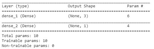
The preceding output confirms our discussion in the previous section: that there will be a total of six parameters in the connection from the input layer to the hidden layer—three weights and three bias terms—we have a total of six parameters corresponding to the three hidden units. In addition, three weights and one bias term connect the hidden layer to the output layer.

4. Compile the model. This ensures that we define the loss function and the optimizer to reduce the loss function and the learning rate corresponding to the optimizer (we will look at different optimizers and loss functions in next chapter):

from keras.optimizers import sgd
sgd = sgd(lr = 0.01)

In the preceding step, we specified that the optimizer is the stochastic gradient descent that we learned about in the previous section and the learning rate is 0.01. Pass the predefined optimizer and its corresponding learning rate as a parameter and reduce the mean squared error value:

model.compile(optimizer=sgd,loss='mean_squared_error')

5. Fit the model. Update the weights so that the model is a better fit:

model.fit(np.array(x), np.array(y), epochs=1, batch_size = 4, verbose=1)

The fit method expects that it receives two NumPy arrays: an input array and the corresponding output array. Note that epochs represents the number of times the total dataset is traversed through, and batch_size represents the number of data points that need to be considered in an iteration of updating the weights. Furthermore, verbose specifies that the output is more detailed, with information about losses in training and test datasets as well as the progress of the model training process.

6. Extract the weight values. The order in which the weight values are presented is obtained by calling the weights method on top of the model, as follows:

model.weights

The order in which weights are obtained is as follows:

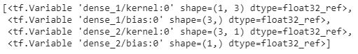
From the preceding output, we see that the order of weights is the three weights (kernel) and three bias terms in the dense_1 layer (which is the connection between the input to the hidden layer) and the three weights (kernel) and one bias term connecting the hidden layer to the dense_2 layer (the output layer).

Now that we understand the order in which weight values are presented, let's extract the values of these weights:

model.get_weights()

Notice that the weights are presented as a list of arrays, where each array corresponds to the value that is specified in the model.weights output.

The output of above lines of code is as follows:

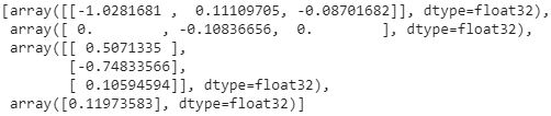
You should notice that the output we are observing here matches with the output we obtaining while hand-building the neural network

7. Predict the output for a new set of input using the predict method:

x1 = [[5],[6]]
model.predict(np.array(x1))

Note that x1 is the variable that holds the values for the new set of examples for which we need to predict the value of the output. Similarly to the fit method, the predict method also expects an array as its input.

The output of preceding code is as follows:

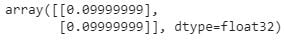
Notice that, while the preceding output is incorrect, the output when we run for 100 epochs is as follows:

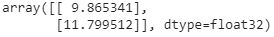
The preceding output will match the expected output (which are 10, 12) as we run for even higher number of epochs.