Data parallelism – the high-level bits

So far, we have discussed the benefits of using data parallelism in machine learning model training, which can tremendously reduce the overall model training time. Now, we need to dive into some fundamental theories about how data parallel training works, such as stochastic gradient descent (SGD) and model synchronization. But before that, let's take a look at the system architecture for data parallel training, and how it is different from single-node training.

The simplified workflow for data parallel training is depicted in the following diagram. We have omitted some technical details during the training phase as we are mainly concerned with the two bandwidths (that is, the data loading bandwidth and the model training bandwidth):

Figure 1.5 – Simplified workflow of data parallel training

As we can see, the main difference between single-node training and data parallel training is that we split the data loading bandwidth between multiple workers/GPUs (shown as blue arrows in the preceding diagram). Therefore, for each GPU involved in the data parallel training job, the difference between its local data loading bandwidth and model training bandwidth is much smaller compared to the single-node case.

At a high level, even though we cannot increase the model training bandwidth on each accelerator due to hardware limitations, we can split and balance the whole data loading bandwidth across multiple accelerators. And this data loading bandwidth split is not only applicable to data parallel training. It can be directly adopted in the data parallel model serving stage.

Note

By decreasing the per-GPU data loading bandwidth, data parallel training mitigates the gap between data loading bandwidth and model training bandwidth on each GPU.

At this point, we should understand how data parallel training increases end-to-end throughput by splitting the data loading bandwidth across multiple accelerators. After each GPU receives its local batch of augmented input data, it will conduct local model training and validation. Here, model validation in data parallel training is the same as in the single-node case (there are some small variations, which we will discuss later) and we mainly focus on the difference at the training stage (excluding validation).

As shown in the following diagram, in the case of a single node, we divide the model training stage into three steps: data loading, training, and model updating. As we mentioned in the Single-node training is too slow section, data loading is for loading new mini-batches of training data. Training is done to conduct forward and backward propagations through the model. Once we've generated gradients during backward propagation, we perform the third step; that is, updating the model parameters:

Figure 1.6 – The three steps in the model training stage

Compared to the data parallel training stage, as shown in the following diagram, there are several major differences:

• First, in data parallel training, different accelerators are trained on different batches of input data (for example, Partition 1 and Partition 2 in the following diagram). Consequently, none of the GPUs can see the full training data. Thus, traditional gradient descent optimization cannot be applied here. We also need to do a stochastic approximation of gradient descent, which can be used in the single-node case. One popular stochastic approximation method is SGD. We will look at this in more detail in the next section.
• Second, in data parallel training, besides the three steps included in single-node training, as shown in the preceding diagram, we have an additional step here called model synchronization, which is shown in the following diagram. Model synchronization is about collecting and aggregating local gradients that have been generated by different nodes. We will learn more about model synchronization later in this book:

Figure 1.7 – Data parallelism procedures within the model training stage

In the next two sections, we will discuss the theoretical details about SGD and model synchronization.

Stochastic gradient descent

In this section, we will discuss why SGD is a must-have for data parallel training and how it works.

In theory, we can use traditional gradient descent (GD) for single-node training. It works as follows:

for i in dataset:
  g_all += g_i
w = w - a*g_all

First, we need to calculate the gradients from each data point of our training dataset, where g_i is the gradients. Here, we calculate this on the i-th training data point. The formal definition of g_i is as follows:

Then, we sum up all the gradients that have been calculated by all the training data points (g_all += g_i) and then do a single step model update with w = w - a*g_all.

However, in data parallel training, each GPU can only see part of (not the full) training dataset, which makes it impossible to use traditional GD optimization since we cannot calculate g_all in this case. Thus, SGD is a must-have. In addition, SGD is also applicable to single-node training. SGD works as follows:

for i in dataset:
  w = w - a*g_i

Basically, instead of updating the model weights (w) after generating the gradients from all the training data, SGD allows for model weights updates using a single or a few training samples (for example, a mini-batch). With this relaxation of model updating restrictions, the workers in data parallel training can update their model weights using their local (not global) training samples.

GD versus SGD

In GD, we need to compute the gradients over all the training data and update the model weights.

In SGD, we compute the gradients over a subset of all the training data and update the model weights.

However, since each worker updates their model weights based on their local training data, the model parameters of different workers can be different after each of the training iterations. Therefore, we need to conduct model synchronization periodically to guarantee that all the workers are on the same page, meaning that they maintain the model parameters after each training iteration.

Model synchronization

As we saw previously, in data parallel training, different workers train their local models using disjointed subsets of the total training data, so the trained model weights may be different. To force all the workers to have the same view of the model parameters, we need to conduct model synchronization.

Let's study this in a simple four-GPU setting, as shown in the following diagram:

Figure 1.8 – Model synchronization in a four-GPU setting

As we can see, we have four GPUs in a data parallel training job. Here, each GPU maintains a copy of the full ML model locally inside its on-device memory.

Let's assume that all the GPUs are initialized with the same model parameters, which is a standard practice, by setting the randomize function with a fixed seed.

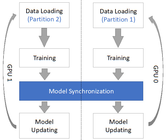
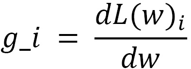
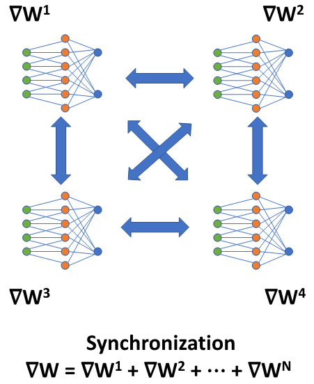
After the first training iteration, each GPU will generate its local gradients as , where i refers to the i-th GPU. Given that they are training on different local training inputs, all the gradients from different GPUs may be different. To guarantee that all four GPUs have the same model updates, we need to conduct model synchronization before the model parameter updates:

Model synchronization does two things:

1. Collects and sums up all the gradients from all the GPUs in use, as shown here:

2. Broadcasts the aggregated gradients to all the GPUs.

Once the model synchronization steps have been completed, we can get the aggregated gradients, , locally on each GPU. Then, we can use these aggregated gradients, , for the model updates, which guarantees that the updated model parameters remain the same after this first data parallel training iteration.

Similarly, in the following training iterations, we conduct model synchronization after each GPU generates its local gradients. So, model synchronization guarantees that the model parameters remain the same after every training iteration in a particular data parallel training job.

For the real system implementations, this model synchronization mainly has two different variations: the parameter server architecture and the All-Reduce architecture, which we will discuss in detail in the next chapter.

So far, we have come across some of the key concepts in data parallel training jobs, such as SGD and model synchronization. Next, we will discuss some important hyperparameters related to data parallel training.