

In this chapter, we will use QGIS to perform many typical geoprocessing and spatial analysis tasks. We will start with raster processing and analysis tasks such as clipping and terrain analysis. We will cover the essentials of converting between raster and vector formats, and then continue with common vector geoprocessing tasks, such as generating heatmaps and calculating area shares within a region. We will also use the Processing modeler to create automated geoprocessing workflows. Finally, we will finish the chapter with examples of how to use the power of spatial databases to analyze spatial data in QGIS.
Raster data, including but not limited to elevation models or remote sensing imagery, is commonly used in many analyses. The following exercises show common raster processing and analysis tasks such as clipping to a certain extent or mask, creating relief and slope rasters from digital elevation models, and using the raster calculator.
A common task in raster processing is clipping a raster with a polygon. This task is well covered by the Clipper tool located in Raster | Extraction | Clipper. This tool supports clipping to a specified extent as well as clipping using a polygon mask layer, as follows:
- Extent can be set manually or by selecting it in the map. To do this, we just click and drag the mouse to open a rectangle in the map area of the main QGIS window.
- A mask layer can be any polygon layer that is currently loaded in the project or any other polygon layer, which can be specified using Select…, right next to the Mask layer drop-down list.
Tip
If we only want to clip a raster to a certain extent (the current map view extent or any other), we can also use the raster Save as... functionality, as shown in Chapter 3, Data Creation and Editing.
For a quick exercise, we will clip the hillshade raster (SR_50M_alaska_nad.tif) using the Alaska Shapefile (both from our sample data) as a mask layer. At the bottom of the window, as shown in the following screenshot, we can see the concrete gdalwarp command that QGIS uses to clip the raster. This is very useful if you also want to learn how to use
GDAL.
Note
In Chapter 2, Viewing Spatial Data, we discussed that GDAL is one of the libraries that QGIS uses to read and process raster data. You can find the documentation of gdalwarp and all other GDAL utility programs at http://www.gdal.org/gdal_utilities.html.

The default No data value is the no data value used in the input dataset or 0 if nothing is specified, but we can override it if necessary. Another good option is to Create an output alpha band, which will set all areas outside the mask to transparent. This will add an extra band to the output raster that will control the transparency of the rendered raster cells.
Tip
A common source of error is forgetting to add the file format extension to the Output file path (in our example, .tif for GeoTIFF). Similarly, you can get errors if you try to overwrite an existing file. In such cases, the best way to fix the error is to either choose a different filename or delete the existing file first.
The resulting layer will be loaded automatically, since we have enabled the Load into canvas when finished option. QGIS should also automatically recognize the alpha layer that we created, and the raster areas that fall outside the Alaska landmass should be transparent, as shown on the right-hand side in the previous screenshot. If, for some reason, QGIS fails to automatically recognize the alpha layer, we can enable it manually using the Transparency band option in the Transparency section of the raster layer's properties, as shown in the following screenshot. This dialog is also the right place to specify any No data value that we might want to be used:

To use terrain analysis tools, we need an elevation raster. If you don't have any at hand, you can simply download a dataset from the NASA Shuttle Radar Topography Mission (SRTM) using http://dwtkns.com/srtm/ or any of the other SRTM download services.
Raster Terrain Analysis can be used to calculate Slope, Aspect, Hillshade, Ruggedness Index, and Relief from elevation rasters. These tools are available through the Raster Terrain Analysis plugin, which comes with QGIS by default, but we have to enable it in the Plugin Manager in order to make it appear in the Raster menu, as shown in the following screenshot:

Terrain Analysis includes the following tools:
- Slope: This tool calculates the slope angle for each cell in degrees (based on the first-order derivative estimation).
- Aspect: This tool calculates the exposition (in degrees and counterclockwise, starting with 0 for north).
- Hillshade: This tool creates a basic hillshade raster with lighted areas and shadows.
- Relief: This tool creates a shaded relief map with varying colors for different elevation ranges.
- Ruggedness Index: This tool calculates the ruggedness of a terrain, which describes how flat or rocky an area is. The index is computed for each cell using the algorithm presented by Riley and others (1999) by summarizing the elevation changes within a 3 x 3 cell grid.
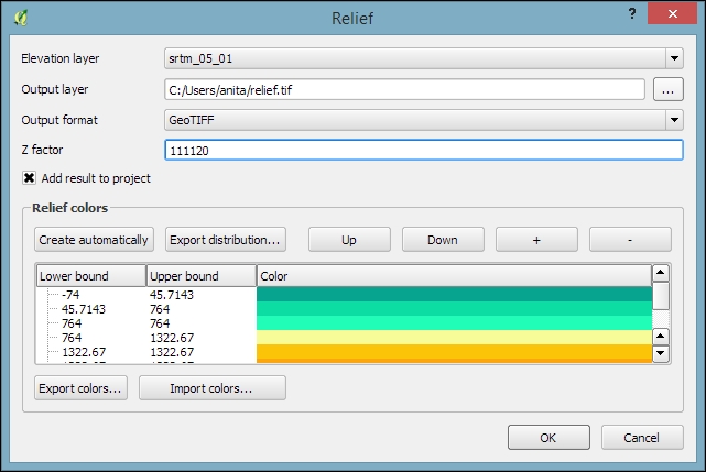
An important element in all terrain analysis tools is the Z factor. The Z factor is used if the x/y units are different from the z (elevation) unit. For example, if we try to create a relief from elevation data where x/y are in degrees and z is in meters, the resulting relief will look grossly exaggerated. The values for the z factor are as follows:
- If x/y and z are either all in meters or all in feet, use the default z factor,
1.0 - If x/y are in degrees and z is in feet, use the z factor
370,400 - If x/y are in degrees and z is in meters, use the z factor
111,120
Since the SRTM rasters are provided in WGS84 EPSG:4326, we need to use a Z factor of 111,120 in our exercise. Let's create a relief! The tool can calculate relief color ranges automatically; we just need to click on Create automatically, as shown in the following screenshot. Of course, we can still edit the elevation ranges' upper and lower bounds as well as the colors by double-clicking on the respective list entry:
While relief maps are three-banded rasters, which are primarily used for visualization purposes, slope rasters are a common intermediate step in spatial analysis workflows. We will now create a slope raster that we can use in our example workflow through the following sections. The resulting slope raster will be loaded in grayscale automatically, as shown in this screenshot:

With the Raster calculator, we can create a new raster layer based on the values in one or more rasters that are loaded in the current QGIS project. To access it, go to Raster | Raster Calculator. All available raster bands are presented in a list in the top-left corner of the dialog using the raster_name@band_number format.
Continuing from our previous exercise in which we created a slope raster, we can, for example, find areas at elevations above 1,000 meters and with a slope of less than 5 degrees using the following expression:
"srtm_05_01@1" > 1000 AND "slope@1" < 5
Cells that meet both criteria of high elevation and evenness will be assigned a value of 1 in the resulting raster, while cells that fail to meet even one criterion will be set to 0. The only bigger areas with a value of 1 are found in the southern part of the raster layer. You can see a section of the resulting raster (displayed in black over the relief layer) to the right-hand side of the following screenshot:

Another typical use case is reclassifying a raster. For example, we might want to reclassify the landcover.img raster in our sample data so that all areas with a landcover class from 1 to 5 get the value 100, areas from 6 to 10 get 101, and areas over 11 get a new value of 102. We will use the following code for this:
("landcover@1" > 0 AND "landcover@1" <= 6 ) * 100
+ ("landcover@1" >= 7 AND "landcover@1" <= 10 ) * 101
+ ("landcover@1" >= 11 ) * 102
The preceding raster calculator expression has three parts, each consisting of a check and a multiplication. For each cell, only one of the three checks can be true, and true is represented as 1. Therefore, if a landcover cell has a value of 4, the first check will be true and the expression will evaluate to 1*100 + 0*101 + 0*102 = 100.
Some analyses require a combination of raster and vector data. In the following exercises, we will use both raster and vector datasets to explain how to convert between these different data types, how to access layer and zonal statistics, and finally how to create a raster heatmap from points.
Tools for converting between raster and vector formats can be accessed by going to Raster | Conversion. These tools are called Rasterize (Vector to raster) and Polygonize (Raster to vector). Like the raster clipper tool that we used before, these tools are also based on GDAL and display the command at the bottom of the dialog.
Polygonize converts a raster into a polygon layer. Depending on the size of the raster, the conversion can take some time. When the process is finished, QGIS will notify us with a popup. For a quick test, we can, for example, convert the reclassified landcover raster to polygons. The resulting vector polygon layer contains multiple polygonal features with a single attribute, which we name lc; it depends on the original raster value, as shown in the following screenshot:

Using the
Rasterize tool is very similar to using the Polygonize tool. The only difference is that we get to specify the size of the resulting raster in pixels/cells. We can also specify the attribute field, which will provide input for the raster cell value, as shown in the next screenshot. In this case, the cat attribute of our alaska.shp dataset is rather meaningless, but you get the idea of how the tool works:

Whenever we get a new dataset, it is useful to examine the layer statistics to get an idea of the data it contains, such as the minimum and maximum values, number of features, and much more. QGIS offers a variety of tools to explore these values.
Raster layer statistics are readily available in the Layer Properties dialog, specifically in the following tabs:
- Metadata: This tab shows the minimum and maximum cell values as well as the mean and the standard deviation of the cell values.
- Histogram: This tab presents the distribution of raster values. Use the mouse to zoom into the histogram to see the details. For example, the following screenshot shows the zoomed-in version of the histogram for our
landcoverdataset:
For vector layers, we can get summary statistics using two tools in Vector | Analysis Tools:
- Basics statistics is very useful for numerical fields. It calculates parameters such as mean and median, min and max, the feature count n, the number of unique values, and so on for all features of a layer or for selected features only.
- List unique values is useful for getting all unique values of a certain field.
In both tools, we can easily copy the results using Ctrl + C and paste them in a text file or spreadsheet. The following image shows examples of exploring the contents of our airports sample dataset:

An alternative to the Basics statistics tool is the Statistics Panel, which you can activate by going to View | Panels | Statistics Panel. As shown in the following screenshot, this panel can be customized to show exactly those statistics that you are interested in:

Instead of computing raster statistics for the entire layer, it is sometimes necessary to compute statistics for selected regions. This is what the Zonal statistics plugin is good for. This plugin is installed by default and can be enabled in the Plugin Manager.
For example, we can compute elevation statistics for areas around each airport using srtm_05_01.tif and airports.shp from our sample data:
- First, we create the analysis areas around each airport using the Vector | Geoprocessing Tools | Buffer(s) tool and a buffer size of
10,000feet. - Before we can use the Zonal statistics plugin, it is important to notice that the buffer layer and the elevation raster use two different CRS (short for Coordinate Reference System). If we simply went ahead, the resulting statistics would be either empty or wrong. Therefore, we need to reproject the buffer layer to the raster CRS (WGS84 EPSG:4326, for details on how to change a layer CRS, see Chapter 3, Data Creation and Editing, in the Reprojecting and converting vector and raster data section).
- Now we can compute the statistics for the analysis areas using the Zonal Statistics tool, which can be accessed by going to Raster | Zonal statistics. Here, we can configure the desired Output column prefix (in our example, we have chosen
elev, which is short for elevation) and the Statistics to calculate (for example,Mean,Minimum, andMaximum), as shown in the following screenshot:
- After you click on OK, the selected statistics are appended to the polygon layer attribute table, as shown in the following screenshot. We can see that Big Mountain AFS is the airport with the highest mean elevation among the four airports that fall within the extent of our elevation raster:

Heatmaps are great for visualizing a distribution of points. To create them, QGIS provides a simple-to-use Heatmap Plugin, which we have to activate in the Plugin Manager, and then we can access it by going to Raster | Heatmap | Heatmap. The plugin offers different Kernel shapes to choose from. The kernel is a moving window of a specific size and shape that moves over an area of points to calculate their local density. Additionally, the plugin allows us to control the output heatmap raster size in cells (using the Rows and Columns settings) as well as the cell size.
Note
Radius determines the distance around each point at which the point will have an influence. Therefore, smaller radius values result in heatmaps that show finer and smaller details, while larger values result in smoother heatmaps with fewer details.
Additionally, Kernel shape controls the rate at which the influence of a point decreases with increasing distance from the point. The kernel shapes that are available in the Heatmap plugin are listed in the following screenshot. For example, a Triweight kernel creates smaller hotspots than the Epanechnikov kernel. For formal definitions of the kernel functions, refer to http://en.wikipedia.org/wiki/Kernel_(statistics).
The following screenshot shows us how to create a heatmap of our airports.shp sample with a kernel radius of 300,000 layer units, which in the case of our airport data is in feet:

By default, the heatmap output will be rendered using the Singleband gray render type (with low raster values in black and high values in white). To change the style to something similar to what you saw in the previous screenshot, you can do the following:
- Change the heatmap raster layer render type to Singleband pseudocolor.
- In the Generate new color map section on the right-hand side of the dialog, select a color map you like, for example, the PuRd color map, as shown in the next screenshot.
- You can enter the Min and Max values for the color map manually, or have them computed by clicking on Load in the Load min/max values section.
Tip
When loading the raster min/max values, keep an eye on the settings. To get the actual min/max values of a raster layer, enable Min/max, Full Extent, and Actual (slower) Accuracy. If you only want the min/max values of the raster section that is currently displayed on the map, use Current Extent instead.
- Click on Classify to add the color map classes to the list on the left-hand side of the dialog.
- Optionally, we can change the color of the first entry (for value 0) to white (by double-clicking on the color in the list) to get a smooth transition from the white map background to our heatmap.

Converting between rasters and vectors
Tools for converting between raster and vector formats can be accessed by going to Raster | Conversion. These tools are called Rasterize (Vector to raster) and Polygonize (Raster to vector). Like the raster clipper tool that we used before, these tools are also based on GDAL and display the command at the bottom of the dialog.
Polygonize converts a raster into a polygon layer. Depending on the size of the raster, the conversion can take some time. When the process is finished, QGIS will notify us with a popup. For a quick test, we can, for example, convert the reclassified landcover raster to polygons. The resulting vector polygon layer contains multiple polygonal features with a single attribute, which we name lc; it depends on the original raster value, as shown in the following screenshot:
Using the
Rasterize tool is very similar to using the Polygonize tool. The only difference is that we get to specify the size of the resulting raster in pixels/cells. We can also specify the attribute field, which will provide input for the raster cell value, as shown in the next screenshot. In this case, the cat attribute of our alaska.shp dataset is rather meaningless, but you get the idea of how the tool works:
Whenever we get a new dataset, it is useful to examine the layer statistics to get an idea of the data it contains, such as the minimum and maximum values, number of features, and much more. QGIS offers a variety of tools to explore these values.
Raster layer statistics are readily available in the Layer Properties dialog, specifically in the following tabs:
- Metadata: This tab shows the minimum and maximum cell values as well as the mean and the standard deviation of the cell values.
- Histogram: This tab presents the distribution of raster values. Use the mouse to zoom into the histogram to see the details. For example, the following screenshot shows the zoomed-in version of the histogram for our
landcoverdataset:
For vector layers, we can get summary statistics using two tools in Vector | Analysis Tools:
- Basics statistics is very useful for numerical fields. It calculates parameters such as mean and median, min and max, the feature count n, the number of unique values, and so on for all features of a layer or for selected features only.
- List unique values is useful for getting all unique values of a certain field.
In both tools, we can easily copy the results using Ctrl + C and paste them in a text file or spreadsheet. The following image shows examples of exploring the contents of our airports sample dataset:
An alternative to the Basics statistics tool is the Statistics Panel, which you can activate by going to View | Panels | Statistics Panel. As shown in the following screenshot, this panel can be customized to show exactly those statistics that you are interested in:
Instead of computing raster statistics for the entire layer, it is sometimes necessary to compute statistics for selected regions. This is what the Zonal statistics plugin is good for. This plugin is installed by default and can be enabled in the Plugin Manager.
For example, we can compute elevation statistics for areas around each airport using srtm_05_01.tif and airports.shp from our sample data:
- First, we create the analysis areas around each airport using the Vector | Geoprocessing Tools | Buffer(s) tool and a buffer size of
10,000feet. - Before we can use the Zonal statistics plugin, it is important to notice that the buffer layer and the elevation raster use two different CRS (short for Coordinate Reference System). If we simply went ahead, the resulting statistics would be either empty or wrong. Therefore, we need to reproject the buffer layer to the raster CRS (WGS84 EPSG:4326, for details on how to change a layer CRS, see Chapter 3, Data Creation and Editing, in the Reprojecting and converting vector and raster data section).
- Now we can compute the statistics for the analysis areas using the Zonal Statistics tool, which can be accessed by going to Raster | Zonal statistics. Here, we can configure the desired Output column prefix (in our example, we have chosen
elev, which is short for elevation) and the Statistics to calculate (for example,Mean,Minimum, andMaximum), as shown in the following screenshot: - After you click on OK, the selected statistics are appended to the polygon layer attribute table, as shown in the following screenshot. We can see that Big Mountain AFS is the airport with the highest mean elevation among the four airports that fall within the extent of our elevation raster:
Heatmaps are great for visualizing a distribution of points. To create them, QGIS provides a simple-to-use Heatmap Plugin, which we have to activate in the Plugin Manager, and then we can access it by going to Raster | Heatmap | Heatmap. The plugin offers different Kernel shapes to choose from. The kernel is a moving window of a specific size and shape that moves over an area of points to calculate their local density. Additionally, the plugin allows us to control the output heatmap raster size in cells (using the Rows and Columns settings) as well as the cell size.
Note
Radius determines the distance around each point at which the point will have an influence. Therefore, smaller radius values result in heatmaps that show finer and smaller details, while larger values result in smoother heatmaps with fewer details.
Additionally, Kernel shape controls the rate at which the influence of a point decreases with increasing distance from the point. The kernel shapes that are available in the Heatmap plugin are listed in the following screenshot. For example, a Triweight kernel creates smaller hotspots than the Epanechnikov kernel. For formal definitions of the kernel functions, refer to http://en.wikipedia.org/wiki/Kernel_(statistics).
The following screenshot shows us how to create a heatmap of our airports.shp sample with a kernel radius of 300,000 layer units, which in the case of our airport data is in feet:
By default, the heatmap output will be rendered using the Singleband gray render type (with low raster values in black and high values in white). To change the style to something similar to what you saw in the previous screenshot, you can do the following:
- Change the heatmap raster layer render type to Singleband pseudocolor.
- In the Generate new color map section on the right-hand side of the dialog, select a color map you like, for example, the PuRd color map, as shown in the next screenshot.
- You can enter the Min and Max values for the color map manually, or have them computed by clicking on Load in the Load min/max values section.
Tip
When loading the raster min/max values, keep an eye on the settings. To get the actual min/max values of a raster layer, enable Min/max, Full Extent, and Actual (slower) Accuracy. If you only want the min/max values of the raster section that is currently displayed on the map, use Current Extent instead.
- Click on Classify to add the color map classes to the list on the left-hand side of the dialog.
- Optionally, we can change the color of the first entry (for value 0) to white (by double-clicking on the color in the list) to get a smooth transition from the white map background to our heatmap.
Accessing raster and vector layer statistics
Whenever we get a new dataset, it is useful to examine the layer statistics to get an idea of the data it contains, such as the minimum and maximum values, number of features, and much more. QGIS offers a variety of tools to explore these values.
Raster layer statistics are readily available in the Layer Properties dialog, specifically in the following tabs:
- Metadata: This tab shows the minimum and maximum cell values as well as the mean and the standard deviation of the cell values.
- Histogram: This tab presents the distribution of raster values. Use the mouse to zoom into the histogram to see the details. For example, the following screenshot shows the zoomed-in version of the histogram for our
landcoverdataset:
For vector layers, we can get summary statistics using two tools in Vector | Analysis Tools:
- Basics statistics is very useful for numerical fields. It calculates parameters such as mean and median, min and max, the feature count n, the number of unique values, and so on for all features of a layer or for selected features only.
- List unique values is useful for getting all unique values of a certain field.
In both tools, we can easily copy the results using Ctrl + C and paste them in a text file or spreadsheet. The following image shows examples of exploring the contents of our airports sample dataset:
An alternative to the Basics statistics tool is the Statistics Panel, which you can activate by going to View | Panels | Statistics Panel. As shown in the following screenshot, this panel can be customized to show exactly those statistics that you are interested in:
Instead of computing raster statistics for the entire layer, it is sometimes necessary to compute statistics for selected regions. This is what the Zonal statistics plugin is good for. This plugin is installed by default and can be enabled in the Plugin Manager.
For example, we can compute elevation statistics for areas around each airport using srtm_05_01.tif and airports.shp from our sample data:
- First, we create the analysis areas around each airport using the Vector | Geoprocessing Tools | Buffer(s) tool and a buffer size of
10,000feet. - Before we can use the Zonal statistics plugin, it is important to notice that the buffer layer and the elevation raster use two different CRS (short for Coordinate Reference System). If we simply went ahead, the resulting statistics would be either empty or wrong. Therefore, we need to reproject the buffer layer to the raster CRS (WGS84 EPSG:4326, for details on how to change a layer CRS, see Chapter 3, Data Creation and Editing, in the Reprojecting and converting vector and raster data section).
- Now we can compute the statistics for the analysis areas using the Zonal Statistics tool, which can be accessed by going to Raster | Zonal statistics. Here, we can configure the desired Output column prefix (in our example, we have chosen
elev, which is short for elevation) and the Statistics to calculate (for example,Mean,Minimum, andMaximum), as shown in the following screenshot: - After you click on OK, the selected statistics are appended to the polygon layer attribute table, as shown in the following screenshot. We can see that Big Mountain AFS is the airport with the highest mean elevation among the four airports that fall within the extent of our elevation raster:
Heatmaps are great for visualizing a distribution of points. To create them, QGIS provides a simple-to-use Heatmap Plugin, which we have to activate in the Plugin Manager, and then we can access it by going to Raster | Heatmap | Heatmap. The plugin offers different Kernel shapes to choose from. The kernel is a moving window of a specific size and shape that moves over an area of points to calculate their local density. Additionally, the plugin allows us to control the output heatmap raster size in cells (using the Rows and Columns settings) as well as the cell size.
Note
Radius determines the distance around each point at which the point will have an influence. Therefore, smaller radius values result in heatmaps that show finer and smaller details, while larger values result in smoother heatmaps with fewer details.
Additionally, Kernel shape controls the rate at which the influence of a point decreases with increasing distance from the point. The kernel shapes that are available in the Heatmap plugin are listed in the following screenshot. For example, a Triweight kernel creates smaller hotspots than the Epanechnikov kernel. For formal definitions of the kernel functions, refer to http://en.wikipedia.org/wiki/Kernel_(statistics).
The following screenshot shows us how to create a heatmap of our airports.shp sample with a kernel radius of 300,000 layer units, which in the case of our airport data is in feet:
By default, the heatmap output will be rendered using the Singleband gray render type (with low raster values in black and high values in white). To change the style to something similar to what you saw in the previous screenshot, you can do the following:
- Change the heatmap raster layer render type to Singleband pseudocolor.
- In the Generate new color map section on the right-hand side of the dialog, select a color map you like, for example, the PuRd color map, as shown in the next screenshot.
- You can enter the Min and Max values for the color map manually, or have them computed by clicking on Load in the Load min/max values section.
Tip
When loading the raster min/max values, keep an eye on the settings. To get the actual min/max values of a raster layer, enable Min/max, Full Extent, and Actual (slower) Accuracy. If you only want the min/max values of the raster section that is currently displayed on the map, use Current Extent instead.
- Click on Classify to add the color map classes to the list on the left-hand side of the dialog.
- Optionally, we can change the color of the first entry (for value 0) to white (by double-clicking on the color in the list) to get a smooth transition from the white map background to our heatmap.
Computing zonal statistics
Instead of computing raster statistics for the entire layer, it is sometimes necessary to compute statistics for selected regions. This is what the Zonal statistics plugin is good for. This plugin is installed by default and can be enabled in the Plugin Manager.
For example, we can compute elevation statistics for areas around each airport using srtm_05_01.tif and airports.shp from our sample data:
- First, we create the analysis areas around each airport using the Vector | Geoprocessing Tools | Buffer(s) tool and a buffer size of
10,000feet. - Before we can use the Zonal statistics plugin, it is important to notice that the buffer layer and the elevation raster use two different CRS (short for Coordinate Reference System). If we simply went ahead, the resulting statistics would be either empty or wrong. Therefore, we need to reproject the buffer layer to the raster CRS (WGS84 EPSG:4326, for details on how to change a layer CRS, see Chapter 3, Data Creation and Editing, in the Reprojecting and converting vector and raster data section).
- Now we can compute the statistics for the analysis areas using the Zonal Statistics tool, which can be accessed by going to Raster | Zonal statistics. Here, we can configure the desired Output column prefix (in our example, we have chosen
elev, which is short for elevation) and the Statistics to calculate (for example,Mean,Minimum, andMaximum), as shown in the following screenshot: - After you click on OK, the selected statistics are appended to the polygon layer attribute table, as shown in the following screenshot. We can see that Big Mountain AFS is the airport with the highest mean elevation among the four airports that fall within the extent of our elevation raster:
Heatmaps are great for visualizing a distribution of points. To create them, QGIS provides a simple-to-use Heatmap Plugin, which we have to activate in the Plugin Manager, and then we can access it by going to Raster | Heatmap | Heatmap. The plugin offers different Kernel shapes to choose from. The kernel is a moving window of a specific size and shape that moves over an area of points to calculate their local density. Additionally, the plugin allows us to control the output heatmap raster size in cells (using the Rows and Columns settings) as well as the cell size.
Note
Radius determines the distance around each point at which the point will have an influence. Therefore, smaller radius values result in heatmaps that show finer and smaller details, while larger values result in smoother heatmaps with fewer details.
Additionally, Kernel shape controls the rate at which the influence of a point decreases with increasing distance from the point. The kernel shapes that are available in the Heatmap plugin are listed in the following screenshot. For example, a Triweight kernel creates smaller hotspots than the Epanechnikov kernel. For formal definitions of the kernel functions, refer to http://en.wikipedia.org/wiki/Kernel_(statistics).
The following screenshot shows us how to create a heatmap of our airports.shp sample with a kernel radius of 300,000 layer units, which in the case of our airport data is in feet:
By default, the heatmap output will be rendered using the Singleband gray render type (with low raster values in black and high values in white). To change the style to something similar to what you saw in the previous screenshot, you can do the following:
- Change the heatmap raster layer render type to Singleband pseudocolor.
- In the Generate new color map section on the right-hand side of the dialog, select a color map you like, for example, the PuRd color map, as shown in the next screenshot.
- You can enter the Min and Max values for the color map manually, or have them computed by clicking on Load in the Load min/max values section.
Tip
When loading the raster min/max values, keep an eye on the settings. To get the actual min/max values of a raster layer, enable Min/max, Full Extent, and Actual (slower) Accuracy. If you only want the min/max values of the raster section that is currently displayed on the map, use Current Extent instead.
- Click on Classify to add the color map classes to the list on the left-hand side of the dialog.
- Optionally, we can change the color of the first entry (for value 0) to white (by double-clicking on the color in the list) to get a smooth transition from the white map background to our heatmap.
Creating a heatmap from points
Heatmaps are great for visualizing a distribution of points. To create them, QGIS provides a simple-to-use Heatmap Plugin, which we have to activate in the Plugin Manager, and then we can access it by going to Raster | Heatmap | Heatmap. The plugin offers different Kernel shapes to choose from. The kernel is a moving window of a specific size and shape that moves over an area of points to calculate their local density. Additionally, the plugin allows us to control the output heatmap raster size in cells (using the Rows and Columns settings) as well as the cell size.
Note
Radius determines the distance around each point at which the point will have an influence. Therefore, smaller radius values result in heatmaps that show finer and smaller details, while larger values result in smoother heatmaps with fewer details.
Additionally, Kernel shape controls the rate at which the influence of a point decreases with increasing distance from the point. The kernel shapes that are available in the Heatmap plugin are listed in the following screenshot. For example, a Triweight kernel creates smaller hotspots than the Epanechnikov kernel. For formal definitions of the kernel functions, refer to http://en.wikipedia.org/wiki/Kernel_(statistics).
The following screenshot shows us how to create a heatmap of our airports.shp sample with a kernel radius of 300,000 layer units, which in the case of our airport data is in feet:
By default, the heatmap output will be rendered using the Singleband gray render type (with low raster values in black and high values in white). To change the style to something similar to what you saw in the previous screenshot, you can do the following:
- Change the heatmap raster layer render type to Singleband pseudocolor.
- In the Generate new color map section on the right-hand side of the dialog, select a color map you like, for example, the PuRd color map, as shown in the next screenshot.
- You can enter the Min and Max values for the color map manually, or have them computed by clicking on Load in the Load min/max values section.
Tip
When loading the raster min/max values, keep an eye on the settings. To get the actual min/max values of a raster layer, enable Min/max, Full Extent, and Actual (slower) Accuracy. If you only want the min/max values of the raster section that is currently displayed on the map, use Current Extent instead.
- Click on Classify to add the color map classes to the list on the left-hand side of the dialog.
- Optionally, we can change the color of the first entry (for value 0) to white (by double-clicking on the color in the list) to get a smooth transition from the white map background to our heatmap.
The most comprehensive set of spatial analysis tools is accessible via the Processing plugin, which we can enable in the Plugin Manager. When this plugin is enabled, we find a Processing menu, where we can activate the Toolbox, as shown in the following screenshot. In the toolbox, it is easy to find spatial analysis tools by their name thanks to the dynamic Search box at the top. This makes finding tools in the toolbox easier than in the Vector or Raster menu. Another advantage of getting accustomed to the Processing tools is that they can be automated in Python and in geoprocessing models.

In the following sections, we will cover a selection of the available geoprocessing tools and see how we can use the modeler to automate our tasks.
Finding nearest neighbors, for example, the airport nearest to a populated place, is a common task in geoprocessing. To find the nearest neighbor and create connections between input features and their nearest neighbor in another layer, we can use the Distance to nearest hub tool.
As shown in the next screenshot, we use the populated places as Source points layer and the airports as the Destination hubs layer. The Hub layer name attribute will be added to the result's attribute table to identify the nearest feature. Therefore, we select NAME to add the airport name to the populated places. There are two options for Output shape type:
- Point: This option creates a point output layer with all points of the source point layer, with new attributes for the nearest hub feature and the distance to it
- Line to hub: This option creates a line output layer with connections between all points of the source point layer and their corresponding nearest hub feature
It is recommended that you use Layer units as Measurement unit to avoid potential issues with wrong measurements:

It is often necessary to be able to convert between points, lines, and polygons, for example, to create lines from a series of points, or to extract the nodes of polygons and create a new point layer out of them. There are many tools that cover these different use cases. The following table provides an overview of the tools that are available in the Processing toolbox for conversion between points, lines, and polygons:
|
To points |
To lines |
To polygons | |
|---|---|---|---|
|
From points |
Points to path |
Convex hull Concave hull | |
|
From lines |
Extract nodes |
Lines to polygons Convex hull | |
|
From polygons |
Extract nodes Polygon centroids (Random points inside a polygon) |
Polygons to lines |
In general, it is easier to convert more complex representations to simpler ones (polygons to lines, polygons to points, or lines to points) than conversion in the other direction (points to lines, points to polygons, or lines to polygons). Here is a short overview of these tools:
- Extract nodes: This is a very straightforward tool. It takes one input layer with lines or polygons and creates a point layer that contains all the input geometry nodes. The resulting points contain all the attributes of the original line or polygon feature.
- Polygon centroids: This tool creates one centroid per polygon or multipolygon. It is worth noting that it does not ensure that the centroid falls within the polygon. For concave polygons, multipolygons, and polygons with holes, the centroid can therefore fall outside the polygon.
- Random points inside polygon: This tool creates a certain number of points at random locations inside the polygon.
- Points to path: To be able to create lines from points, the point layer needs attributes that identify the line (Group field) and the order of points in the line (Order field), as shown in this screenshot:

- Convex hull: This tool creates a convex hull around the input points or lines. The convex hull can be imagined as an area that contains all the input points as well as all the connections between the input points.
- Concave hull: This tool creates a concave hull around the input points. The concave hull is a polygon that represents the area occupied by the input points. The concave hull is equal to or smaller than the convex hull. In this tool, we can control the level of detail of the concave hull by changing the Threshold parameter between
0(very detailed) and1(which is equivalent to the convex hull). The following screenshot shows a comparison between convex and concave hulls (with the threshold set to0.3) around our airport data:
- Lines to polygon: Finally, this tool can create polygons from lines that enclose an area. Make sure that there are no gaps between the lines. Otherwise, it will not work.
One common spatial analysis task is to identify features in the proximity of certain other features. One example would be to find all airports near rivers. Using airports.shp and majrivers.shp from our sample data, we can find airports within 5,000 feet of a river by using a combination of the Fixed distance buffer and Select by location tools. Use the search box to find the tools in the Processing Toolbox. The tool configurations for this example are shown in the following screenshot:

After buffering the airport point locations, the Select by location tool selects all the airport buffers that intersect a river. As a result, 14 out of the 76 airports are selected. This information is displayed in the information area at the bottom of the QGIS main window, as shown in this screenshot:

If you ever forget which settings you used or need to check whether you have used the correct input layer, you can go to Processing | History. The ALGORITHM section lists all the algorithms that we have been running as well as the used settings, as shown in the following screenshot:

The commands listed under ALGORITHM can also be used to call Processing tools from the QGIS Python console, which can be activated by going to Plugins | Python Console. The Python commands shown in the following screenshot run the buffer algorithm (processing.runalg) and load the result into the map (processing.load):

Another common task is to sample a raster at specific point locations. Using Processing, we can solve this problem with a GRASS tool called v.sample. To use GRASS tools, make sure that GRASS is installed and Processing is configured correctly under Processing | Options and configuration. On an OSGeo4W default system, the configuration will look like what is shown here:

Note
At the time of writing this book, GRASS 7.0.3RC1 is available in OSGeo4W. As shown in the previous screenshot, there is also support for the previous GRASS version 6.x, and Processing can be configured to use its algorithms as well. In the toolbox, you will find the algorithms under GRASS GIS 7 commands and GRASS commands (for GRASS 6.x).
For this exercise, let's imagine we want to sample the landcover layer at the airport locations of our sample data. All we have to do is specify the vector layer containing the sample points and the raster layer that should be sampled. For this example, we can leave all other settings at their default values, as shown in the following screenshot. The tool not only samples the raster but also compares point attributes with the sampled raster value. However, we don't need this comparison in our current example:

Mapping the density of points using a hexagonal grid has become quite a popular alternative to creating heatmaps. Processing offers us a fast way to create such an analysis. There is already a pre-made script called Hex grid from layer bounds, which is available through the Processing scripts collection and can be downloaded using the Get scripts from on-line scripts collection tool. As you can see in the following screenshot, you just need to enable the script by ticking the checkbox and clicking OK:

Then, we can use this script to create a hexagonal grid that covers all points in the input layer. The dataset of populated places (popp.shp), is a good sample dataset for this exercise. Once the grid is ready, we can run Count points in polygon to calculate the statistics. The number of points will be stored in the NUMPOINTS column if you use the settings shown in the following screenshot:

Another spatial analysis task we often encounter is calculating area shares within a certain region, for example, landcover shares along one specific river. Using majrivers.shp and trees.shp, we can calculate the share of wooded area in a 10,000-foot-wide strip of land along the Susitna River:
- We first define the analysis region by selecting the river and buffering it.
To select the Susitna River, we use the Select by attribute tool. After running the tool, you should see that our river of interest is selected and highlighted.
- Then we can use the Fixed distance buffer tool to get the area within 5,000 feet along the river. Note that the Dissolve result option should be enabled to ensure that the buffer result is one continuous polygon, as shown in the following screenshot:

- Next, we calculate the size of the strip of land around our river. This can be done using the Export/Add geometry columns tool, which adds the area and perimeter to the attribute table.
- Then, we can calculate the Intersection between the area along the river and the wooded areas in
trees.shp, as shown in the following screenshot. The result of this operation is a layer that contains only those wooded areas within the river buffer.
- Using the Dissolve tool, we can recombine all areas from the intersection results into one big polygon that represents the total wooded area around the river. Note how we use the Unique ID field
VEGDESCto only combine areas with the same vegetation in order not to mix deciduous and mixed trees. - Finally, we can calculate the final share of wooded area using the Advanced Python field calculator. The formula
value = $geom.area()/<area>divides the area of the final polygon ($geom.area()) by the value in theareaattribute (<area>), which we created earlier by running Export/Add geometry columns. As shown in the following screenshot, this calculation results in a wood share of 0.31601 for Deciduous and 0.09666 for Mixed Trees. Therefore, we can conclude that in total, 41.27 percent of the land along the Susitna River is wooded:
Sometimes, we want to run the same tool repeatedly but with slightly different settings. For this use case, Processing offers the Batch Processing functionality. Let's use this tool to extract some samples from our airports layer using the Random extract tool:
- To access the batch processing functionality, right-click on the Random extract tool in the toolbox and select Execute as batch process. This will open the Batch Processing dialog.
- Next, we configure the Input layer by clicking on the ... button and selecting Select from open layers, as shown in the following screenshot:

- This will open a small dialog in which we can select the
airportslayer and click on OK. - To automatically fill in the other rows with the same input layer, we can double-click on the table header of the corresponding column (which reads Input layer).
- Next, we configure the Method by selecting the Percentage of selected features option and again double-clicking on the respective table header to auto-fill the remaining rows.
- The next parameter controls the Number/percentage of selected features. For our exercise, we configure 10, 20, and 30 percent.
- Last but not least, we need to configure the output files in the Extracted (random) column. Click on the ... button, which will open a file dialog. There, you can select the save location and filename (for example,
extract) and click on Save. - This will open the Autofill settings dialog, which helps us to automatically create distinct filenames for each run. Using the Fill with parameter values mode with the Number/percentage of selected features parameter will automatically append our parameter values (10, 20, and 30, respectively) to the filename. This will result in
extract10,extract20, andextract30, as shown in the following screenshot:
- Once everything is configured, click on the Run button and wait for all the batch instructions to be processed and the results to be loaded into the project.
Using the graphical modeler, we can turn entire geoprocessing and analysis workflows into automated models. We can then use these models to run complex geoprocessing tasks that involve multiple different tools in one go. To create a model, we go to Processing | Graphical modeler to open the modeler, where we can select from different Inputs and Algorithms for our model.
Let's create a model that automates the creation of hexagonal heatmaps!
- By double-clicking on the Vector layer entry in the Inputs list, we can add an input field for the point layer. It's a good idea to use descriptive parameter names (for example,
hex cell sizeinstead of justsizefor the parameter that controls the size of the hexagonal grid cells) so that we can recognize which input is first and which is later in the model. It is also useful to restrict the Shape type field wherever appropriate. In our example, we restrict the input to Point layers. This will enable Processing to pre-filter the available layers and present us only the layers of the correct type. - The second input that we need is a Number field to specify the desired hexagonal cell size, as shown in this screenshot:

- After adding the inputs, we can now continue creating the model by assembling the algorithms. In the Algorithms section, we can use the filter at the top to narrow down our search for the correct algorithm. To add an algorithm to the model, we simply double-click on the entry in the list of algorithms. This opens the algorithm dialog, where we have to specify the inputs and further algorithm-specific parameters.
- In our example, we want to use the point vector layer as the input layer and the number input hex cell size as the cellsize parameter. We can access the available inputs through the drop-down list, as shown in the following screenshot. Alternatively, it's possible to hardcode parameters such as the cell size by typing the desired value in the input field:

- The final model will look like this:

- To finish the model, we need to enter a model name (for example,
Create hexagonal heatmap) and a group name (for example,Learning QGIS). Processing will use the group name to organize all the models that we create into different toolbox groups. Once we have picked a name and group, we can save the model and then run it. - After closing the modeler, we can run the saved models from the toolbox like any other tool. It is even possible to use one model as a building block for another model.
Another useful feature is that we can specify a layer style that needs to be applied to the processing results automatically. This default style can be set using Edit rendering styles for outputs in the context menu of the created model in the toolbox, as shown in the following screenshot:

Models can easily be copied from one QGIS installation to another and shared with other users. To ensure the usability of the model, it is a good idea to write a short documentation. Processing provides a convenient Help editor; it can be accessed by clicking on the Edit model help button in the Processing modeler, as shown in this screenshot:

By default, the .model files are stored in your user directory. On Windows, it is C:\Users\<your_user_name>\.qgis2\processing\models, and on Linux and OS X, it is ~/.qgis2/processing/models.
You can copy these files and share them with others. To load a model from a file, use the loading tool by going to Models | Tools | Add model from file in the Processing Toolbox.
Finding nearest neighbors
Finding nearest neighbors, for example, the airport nearest to a populated place, is a common task in geoprocessing. To find the nearest neighbor and create connections between input features and their nearest neighbor in another layer, we can use the Distance to nearest hub tool.
As shown in the next screenshot, we use the populated places as Source points layer and the airports as the Destination hubs layer. The Hub layer name attribute will be added to the result's attribute table to identify the nearest feature. Therefore, we select NAME to add the airport name to the populated places. There are two options for Output shape type:
- Point: This option creates a point output layer with all points of the source point layer, with new attributes for the nearest hub feature and the distance to it
- Line to hub: This option creates a line output layer with connections between all points of the source point layer and their corresponding nearest hub feature
It is recommended that you use Layer units as Measurement unit to avoid potential issues with wrong measurements:
It is often necessary to be able to convert between points, lines, and polygons, for example, to create lines from a series of points, or to extract the nodes of polygons and create a new point layer out of them. There are many tools that cover these different use cases. The following table provides an overview of the tools that are available in the Processing toolbox for conversion between points, lines, and polygons:
|
To points |
To lines |
To polygons | |
|---|---|---|---|
|
From points |
Points to path |
Convex hull Concave hull | |
|
From lines |
Extract nodes |
Lines to polygons Convex hull | |
|
From polygons |
Extract nodes Polygon centroids (Random points inside a polygon) |
Polygons to lines |
In general, it is easier to convert more complex representations to simpler ones (polygons to lines, polygons to points, or lines to points) than conversion in the other direction (points to lines, points to polygons, or lines to polygons). Here is a short overview of these tools:
- Extract nodes: This is a very straightforward tool. It takes one input layer with lines or polygons and creates a point layer that contains all the input geometry nodes. The resulting points contain all the attributes of the original line or polygon feature.
- Polygon centroids: This tool creates one centroid per polygon or multipolygon. It is worth noting that it does not ensure that the centroid falls within the polygon. For concave polygons, multipolygons, and polygons with holes, the centroid can therefore fall outside the polygon.
- Random points inside polygon: This tool creates a certain number of points at random locations inside the polygon.
- Points to path: To be able to create lines from points, the point layer needs attributes that identify the line (Group field) and the order of points in the line (Order field), as shown in this screenshot:
- Convex hull: This tool creates a convex hull around the input points or lines. The convex hull can be imagined as an area that contains all the input points as well as all the connections between the input points.
- Concave hull: This tool creates a concave hull around the input points. The concave hull is a polygon that represents the area occupied by the input points. The concave hull is equal to or smaller than the convex hull. In this tool, we can control the level of detail of the concave hull by changing the Threshold parameter between
0(very detailed) and1(which is equivalent to the convex hull). The following screenshot shows a comparison between convex and concave hulls (with the threshold set to0.3) around our airport data: - Lines to polygon: Finally, this tool can create polygons from lines that enclose an area. Make sure that there are no gaps between the lines. Otherwise, it will not work.
One common spatial analysis task is to identify features in the proximity of certain other features. One example would be to find all airports near rivers. Using airports.shp and majrivers.shp from our sample data, we can find airports within 5,000 feet of a river by using a combination of the Fixed distance buffer and Select by location tools. Use the search box to find the tools in the Processing Toolbox. The tool configurations for this example are shown in the following screenshot:
After buffering the airport point locations, the Select by location tool selects all the airport buffers that intersect a river. As a result, 14 out of the 76 airports are selected. This information is displayed in the information area at the bottom of the QGIS main window, as shown in this screenshot:
If you ever forget which settings you used or need to check whether you have used the correct input layer, you can go to Processing | History. The ALGORITHM section lists all the algorithms that we have been running as well as the used settings, as shown in the following screenshot:
The commands listed under ALGORITHM can also be used to call Processing tools from the QGIS Python console, which can be activated by going to Plugins | Python Console. The Python commands shown in the following screenshot run the buffer algorithm (processing.runalg) and load the result into the map (processing.load):
Another common task is to sample a raster at specific point locations. Using Processing, we can solve this problem with a GRASS tool called v.sample. To use GRASS tools, make sure that GRASS is installed and Processing is configured correctly under Processing | Options and configuration. On an OSGeo4W default system, the configuration will look like what is shown here:
Note
At the time of writing this book, GRASS 7.0.3RC1 is available in OSGeo4W. As shown in the previous screenshot, there is also support for the previous GRASS version 6.x, and Processing can be configured to use its algorithms as well. In the toolbox, you will find the algorithms under GRASS GIS 7 commands and GRASS commands (for GRASS 6.x).
For this exercise, let's imagine we want to sample the landcover layer at the airport locations of our sample data. All we have to do is specify the vector layer containing the sample points and the raster layer that should be sampled. For this example, we can leave all other settings at their default values, as shown in the following screenshot. The tool not only samples the raster but also compares point attributes with the sampled raster value. However, we don't need this comparison in our current example:
Mapping the density of points using a hexagonal grid has become quite a popular alternative to creating heatmaps. Processing offers us a fast way to create such an analysis. There is already a pre-made script called Hex grid from layer bounds, which is available through the Processing scripts collection and can be downloaded using the Get scripts from on-line scripts collection tool. As you can see in the following screenshot, you just need to enable the script by ticking the checkbox and clicking OK:
Then, we can use this script to create a hexagonal grid that covers all points in the input layer. The dataset of populated places (popp.shp), is a good sample dataset for this exercise. Once the grid is ready, we can run Count points in polygon to calculate the statistics. The number of points will be stored in the NUMPOINTS column if you use the settings shown in the following screenshot:
Another spatial analysis task we often encounter is calculating area shares within a certain region, for example, landcover shares along one specific river. Using majrivers.shp and trees.shp, we can calculate the share of wooded area in a 10,000-foot-wide strip of land along the Susitna River:
- We first define the analysis region by selecting the river and buffering it.
To select the Susitna River, we use the Select by attribute tool. After running the tool, you should see that our river of interest is selected and highlighted.
- Then we can use the Fixed distance buffer tool to get the area within 5,000 feet along the river. Note that the Dissolve result option should be enabled to ensure that the buffer result is one continuous polygon, as shown in the following screenshot:
- Next, we calculate the size of the strip of land around our river. This can be done using the Export/Add geometry columns tool, which adds the area and perimeter to the attribute table.
- Then, we can calculate the Intersection between the area along the river and the wooded areas in
trees.shp, as shown in the following screenshot. The result of this operation is a layer that contains only those wooded areas within the river buffer. - Using the Dissolve tool, we can recombine all areas from the intersection results into one big polygon that represents the total wooded area around the river. Note how we use the Unique ID field
VEGDESCto only combine areas with the same vegetation in order not to mix deciduous and mixed trees. - Finally, we can calculate the final share of wooded area using the Advanced Python field calculator. The formula
value = $geom.area()/<area>divides the area of the final polygon ($geom.area()) by the value in theareaattribute (<area>), which we created earlier by running Export/Add geometry columns. As shown in the following screenshot, this calculation results in a wood share of 0.31601 for Deciduous and 0.09666 for Mixed Trees. Therefore, we can conclude that in total, 41.27 percent of the land along the Susitna River is wooded:
Sometimes, we want to run the same tool repeatedly but with slightly different settings. For this use case, Processing offers the Batch Processing functionality. Let's use this tool to extract some samples from our airports layer using the Random extract tool:
- To access the batch processing functionality, right-click on the Random extract tool in the toolbox and select Execute as batch process. This will open the Batch Processing dialog.
- Next, we configure the Input layer by clicking on the ... button and selecting Select from open layers, as shown in the following screenshot:
- This will open a small dialog in which we can select the
airportslayer and click on OK. - To automatically fill in the other rows with the same input layer, we can double-click on the table header of the corresponding column (which reads Input layer).
- Next, we configure the Method by selecting the Percentage of selected features option and again double-clicking on the respective table header to auto-fill the remaining rows.
- The next parameter controls the Number/percentage of selected features. For our exercise, we configure 10, 20, and 30 percent.
- Last but not least, we need to configure the output files in the Extracted (random) column. Click on the ... button, which will open a file dialog. There, you can select the save location and filename (for example,
extract) and click on Save. - This will open the Autofill settings dialog, which helps us to automatically create distinct filenames for each run. Using the Fill with parameter values mode with the Number/percentage of selected features parameter will automatically append our parameter values (10, 20, and 30, respectively) to the filename. This will result in
extract10,extract20, andextract30, as shown in the following screenshot: - Once everything is configured, click on the Run button and wait for all the batch instructions to be processed and the results to be loaded into the project.
Using the graphical modeler, we can turn entire geoprocessing and analysis workflows into automated models. We can then use these models to run complex geoprocessing tasks that involve multiple different tools in one go. To create a model, we go to Processing | Graphical modeler to open the modeler, where we can select from different Inputs and Algorithms for our model.
Let's create a model that automates the creation of hexagonal heatmaps!
- By double-clicking on the Vector layer entry in the Inputs list, we can add an input field for the point layer. It's a good idea to use descriptive parameter names (for example,
hex cell sizeinstead of justsizefor the parameter that controls the size of the hexagonal grid cells) so that we can recognize which input is first and which is later in the model. It is also useful to restrict the Shape type field wherever appropriate. In our example, we restrict the input to Point layers. This will enable Processing to pre-filter the available layers and present us only the layers of the correct type. - The second input that we need is a Number field to specify the desired hexagonal cell size, as shown in this screenshot:
- After adding the inputs, we can now continue creating the model by assembling the algorithms. In the Algorithms section, we can use the filter at the top to narrow down our search for the correct algorithm. To add an algorithm to the model, we simply double-click on the entry in the list of algorithms. This opens the algorithm dialog, where we have to specify the inputs and further algorithm-specific parameters.
- In our example, we want to use the point vector layer as the input layer and the number input hex cell size as the cellsize parameter. We can access the available inputs through the drop-down list, as shown in the following screenshot. Alternatively, it's possible to hardcode parameters such as the cell size by typing the desired value in the input field:
- The final model will look like this:
- To finish the model, we need to enter a model name (for example,
Create hexagonal heatmap) and a group name (for example,Learning QGIS). Processing will use the group name to organize all the models that we create into different toolbox groups. Once we have picked a name and group, we can save the model and then run it. - After closing the modeler, we can run the saved models from the toolbox like any other tool. It is even possible to use one model as a building block for another model.
Another useful feature is that we can specify a layer style that needs to be applied to the processing results automatically. This default style can be set using Edit rendering styles for outputs in the context menu of the created model in the toolbox, as shown in the following screenshot:
Models can easily be copied from one QGIS installation to another and shared with other users. To ensure the usability of the model, it is a good idea to write a short documentation. Processing provides a convenient Help editor; it can be accessed by clicking on the Edit model help button in the Processing modeler, as shown in this screenshot:
By default, the .model files are stored in your user directory. On Windows, it is C:\Users\<your_user_name>\.qgis2\processing\models, and on Linux and OS X, it is ~/.qgis2/processing/models.
You can copy these files and share them with others. To load a model from a file, use the loading tool by going to Models | Tools | Add model from file in the Processing Toolbox.
Converting between points, lines, and polygons
It is often necessary to be able to convert between points, lines, and polygons, for example, to create lines from a series of points, or to extract the nodes of polygons and create a new point layer out of them. There are many tools that cover these different use cases. The following table provides an overview of the tools that are available in the Processing toolbox for conversion between points, lines, and polygons:
|
To points |
To lines |
To polygons | |
|---|---|---|---|
|
From points |
Points to path |
Convex hull Concave hull | |
|
From lines |
Extract nodes |
Lines to polygons Convex hull | |
|
From polygons |
Extract nodes Polygon centroids (Random points inside a polygon) |
Polygons to lines |
In general, it is easier to convert more complex representations to simpler ones (polygons to lines, polygons to points, or lines to points) than conversion in the other direction (points to lines, points to polygons, or lines to polygons). Here is a short overview of these tools:
- Extract nodes: This is a very straightforward tool. It takes one input layer with lines or polygons and creates a point layer that contains all the input geometry nodes. The resulting points contain all the attributes of the original line or polygon feature.
- Polygon centroids: This tool creates one centroid per polygon or multipolygon. It is worth noting that it does not ensure that the centroid falls within the polygon. For concave polygons, multipolygons, and polygons with holes, the centroid can therefore fall outside the polygon.
- Random points inside polygon: This tool creates a certain number of points at random locations inside the polygon.
- Points to path: To be able to create lines from points, the point layer needs attributes that identify the line (Group field) and the order of points in the line (Order field), as shown in this screenshot:
- Convex hull: This tool creates a convex hull around the input points or lines. The convex hull can be imagined as an area that contains all the input points as well as all the connections between the input points.
- Concave hull: This tool creates a concave hull around the input points. The concave hull is a polygon that represents the area occupied by the input points. The concave hull is equal to or smaller than the convex hull. In this tool, we can control the level of detail of the concave hull by changing the Threshold parameter between
0(very detailed) and1(which is equivalent to the convex hull). The following screenshot shows a comparison between convex and concave hulls (with the threshold set to0.3) around our airport data: - Lines to polygon: Finally, this tool can create polygons from lines that enclose an area. Make sure that there are no gaps between the lines. Otherwise, it will not work.
One common spatial analysis task is to identify features in the proximity of certain other features. One example would be to find all airports near rivers. Using airports.shp and majrivers.shp from our sample data, we can find airports within 5,000 feet of a river by using a combination of the Fixed distance buffer and Select by location tools. Use the search box to find the tools in the Processing Toolbox. The tool configurations for this example are shown in the following screenshot:
After buffering the airport point locations, the Select by location tool selects all the airport buffers that intersect a river. As a result, 14 out of the 76 airports are selected. This information is displayed in the information area at the bottom of the QGIS main window, as shown in this screenshot:
If you ever forget which settings you used or need to check whether you have used the correct input layer, you can go to Processing | History. The ALGORITHM section lists all the algorithms that we have been running as well as the used settings, as shown in the following screenshot:
The commands listed under ALGORITHM can also be used to call Processing tools from the QGIS Python console, which can be activated by going to Plugins | Python Console. The Python commands shown in the following screenshot run the buffer algorithm (processing.runalg) and load the result into the map (processing.load):
Another common task is to sample a raster at specific point locations. Using Processing, we can solve this problem with a GRASS tool called v.sample. To use GRASS tools, make sure that GRASS is installed and Processing is configured correctly under Processing | Options and configuration. On an OSGeo4W default system, the configuration will look like what is shown here:
Note
At the time of writing this book, GRASS 7.0.3RC1 is available in OSGeo4W. As shown in the previous screenshot, there is also support for the previous GRASS version 6.x, and Processing can be configured to use its algorithms as well. In the toolbox, you will find the algorithms under GRASS GIS 7 commands and GRASS commands (for GRASS 6.x).
For this exercise, let's imagine we want to sample the landcover layer at the airport locations of our sample data. All we have to do is specify the vector layer containing the sample points and the raster layer that should be sampled. For this example, we can leave all other settings at their default values, as shown in the following screenshot. The tool not only samples the raster but also compares point attributes with the sampled raster value. However, we don't need this comparison in our current example:
Mapping the density of points using a hexagonal grid has become quite a popular alternative to creating heatmaps. Processing offers us a fast way to create such an analysis. There is already a pre-made script called Hex grid from layer bounds, which is available through the Processing scripts collection and can be downloaded using the Get scripts from on-line scripts collection tool. As you can see in the following screenshot, you just need to enable the script by ticking the checkbox and clicking OK:
Then, we can use this script to create a hexagonal grid that covers all points in the input layer. The dataset of populated places (popp.shp), is a good sample dataset for this exercise. Once the grid is ready, we can run Count points in polygon to calculate the statistics. The number of points will be stored in the NUMPOINTS column if you use the settings shown in the following screenshot:
Another spatial analysis task we often encounter is calculating area shares within a certain region, for example, landcover shares along one specific river. Using majrivers.shp and trees.shp, we can calculate the share of wooded area in a 10,000-foot-wide strip of land along the Susitna River:
- We first define the analysis region by selecting the river and buffering it.
To select the Susitna River, we use the Select by attribute tool. After running the tool, you should see that our river of interest is selected and highlighted.
- Then we can use the Fixed distance buffer tool to get the area within 5,000 feet along the river. Note that the Dissolve result option should be enabled to ensure that the buffer result is one continuous polygon, as shown in the following screenshot:
- Next, we calculate the size of the strip of land around our river. This can be done using the Export/Add geometry columns tool, which adds the area and perimeter to the attribute table.
- Then, we can calculate the Intersection between the area along the river and the wooded areas in
trees.shp, as shown in the following screenshot. The result of this operation is a layer that contains only those wooded areas within the river buffer. - Using the Dissolve tool, we can recombine all areas from the intersection results into one big polygon that represents the total wooded area around the river. Note how we use the Unique ID field
VEGDESCto only combine areas with the same vegetation in order not to mix deciduous and mixed trees. - Finally, we can calculate the final share of wooded area using the Advanced Python field calculator. The formula
value = $geom.area()/<area>divides the area of the final polygon ($geom.area()) by the value in theareaattribute (<area>), which we created earlier by running Export/Add geometry columns. As shown in the following screenshot, this calculation results in a wood share of 0.31601 for Deciduous and 0.09666 for Mixed Trees. Therefore, we can conclude that in total, 41.27 percent of the land along the Susitna River is wooded:
Sometimes, we want to run the same tool repeatedly but with slightly different settings. For this use case, Processing offers the Batch Processing functionality. Let's use this tool to extract some samples from our airports layer using the Random extract tool:
- To access the batch processing functionality, right-click on the Random extract tool in the toolbox and select Execute as batch process. This will open the Batch Processing dialog.
- Next, we configure the Input layer by clicking on the ... button and selecting Select from open layers, as shown in the following screenshot:
- This will open a small dialog in which we can select the
airportslayer and click on OK. - To automatically fill in the other rows with the same input layer, we can double-click on the table header of the corresponding column (which reads Input layer).
- Next, we configure the Method by selecting the Percentage of selected features option and again double-clicking on the respective table header to auto-fill the remaining rows.
- The next parameter controls the Number/percentage of selected features. For our exercise, we configure 10, 20, and 30 percent.
- Last but not least, we need to configure the output files in the Extracted (random) column. Click on the ... button, which will open a file dialog. There, you can select the save location and filename (for example,
extract) and click on Save. - This will open the Autofill settings dialog, which helps us to automatically create distinct filenames for each run. Using the Fill with parameter values mode with the Number/percentage of selected features parameter will automatically append our parameter values (10, 20, and 30, respectively) to the filename. This will result in
extract10,extract20, andextract30, as shown in the following screenshot: - Once everything is configured, click on the Run button and wait for all the batch instructions to be processed and the results to be loaded into the project.
Using the graphical modeler, we can turn entire geoprocessing and analysis workflows into automated models. We can then use these models to run complex geoprocessing tasks that involve multiple different tools in one go. To create a model, we go to Processing | Graphical modeler to open the modeler, where we can select from different Inputs and Algorithms for our model.
Let's create a model that automates the creation of hexagonal heatmaps!
- By double-clicking on the Vector layer entry in the Inputs list, we can add an input field for the point layer. It's a good idea to use descriptive parameter names (for example,
hex cell sizeinstead of justsizefor the parameter that controls the size of the hexagonal grid cells) so that we can recognize which input is first and which is later in the model. It is also useful to restrict the Shape type field wherever appropriate. In our example, we restrict the input to Point layers. This will enable Processing to pre-filter the available layers and present us only the layers of the correct type. - The second input that we need is a Number field to specify the desired hexagonal cell size, as shown in this screenshot:
- After adding the inputs, we can now continue creating the model by assembling the algorithms. In the Algorithms section, we can use the filter at the top to narrow down our search for the correct algorithm. To add an algorithm to the model, we simply double-click on the entry in the list of algorithms. This opens the algorithm dialog, where we have to specify the inputs and further algorithm-specific parameters.
- In our example, we want to use the point vector layer as the input layer and the number input hex cell size as the cellsize parameter. We can access the available inputs through the drop-down list, as shown in the following screenshot. Alternatively, it's possible to hardcode parameters such as the cell size by typing the desired value in the input field:
- The final model will look like this:
- To finish the model, we need to enter a model name (for example,
Create hexagonal heatmap) and a group name (for example,Learning QGIS). Processing will use the group name to organize all the models that we create into different toolbox groups. Once we have picked a name and group, we can save the model and then run it. - After closing the modeler, we can run the saved models from the toolbox like any other tool. It is even possible to use one model as a building block for another model.
Another useful feature is that we can specify a layer style that needs to be applied to the processing results automatically. This default style can be set using Edit rendering styles for outputs in the context menu of the created model in the toolbox, as shown in the following screenshot:
Models can easily be copied from one QGIS installation to another and shared with other users. To ensure the usability of the model, it is a good idea to write a short documentation. Processing provides a convenient Help editor; it can be accessed by clicking on the Edit model help button in the Processing modeler, as shown in this screenshot:
By default, the .model files are stored in your user directory. On Windows, it is C:\Users\<your_user_name>\.qgis2\processing\models, and on Linux and OS X, it is ~/.qgis2/processing/models.
You can copy these files and share them with others. To load a model from a file, use the loading tool by going to Models | Tools | Add model from file in the Processing Toolbox.
Identifying features in the proximity of other features
One common spatial analysis task is to identify features in the proximity of certain other features. One example would be to find all airports near rivers. Using airports.shp and majrivers.shp from our sample data, we can find airports within 5,000 feet of a river by using a combination of the Fixed distance buffer and Select by location tools. Use the search box to find the tools in the Processing Toolbox. The tool configurations for this example are shown in the following screenshot:
After buffering the airport point locations, the Select by location tool selects all the airport buffers that intersect a river. As a result, 14 out of the 76 airports are selected. This information is displayed in the information area at the bottom of the QGIS main window, as shown in this screenshot:
If you ever forget which settings you used or need to check whether you have used the correct input layer, you can go to Processing | History. The ALGORITHM section lists all the algorithms that we have been running as well as the used settings, as shown in the following screenshot:
The commands listed under ALGORITHM can also be used to call Processing tools from the QGIS Python console, which can be activated by going to Plugins | Python Console. The Python commands shown in the following screenshot run the buffer algorithm (processing.runalg) and load the result into the map (processing.load):
Another common task is to sample a raster at specific point locations. Using Processing, we can solve this problem with a GRASS tool called v.sample. To use GRASS tools, make sure that GRASS is installed and Processing is configured correctly under Processing | Options and configuration. On an OSGeo4W default system, the configuration will look like what is shown here:
Note
At the time of writing this book, GRASS 7.0.3RC1 is available in OSGeo4W. As shown in the previous screenshot, there is also support for the previous GRASS version 6.x, and Processing can be configured to use its algorithms as well. In the toolbox, you will find the algorithms under GRASS GIS 7 commands and GRASS commands (for GRASS 6.x).
For this exercise, let's imagine we want to sample the landcover layer at the airport locations of our sample data. All we have to do is specify the vector layer containing the sample points and the raster layer that should be sampled. For this example, we can leave all other settings at their default values, as shown in the following screenshot. The tool not only samples the raster but also compares point attributes with the sampled raster value. However, we don't need this comparison in our current example:
Mapping the density of points using a hexagonal grid has become quite a popular alternative to creating heatmaps. Processing offers us a fast way to create such an analysis. There is already a pre-made script called Hex grid from layer bounds, which is available through the Processing scripts collection and can be downloaded using the Get scripts from on-line scripts collection tool. As you can see in the following screenshot, you just need to enable the script by ticking the checkbox and clicking OK:
Then, we can use this script to create a hexagonal grid that covers all points in the input layer. The dataset of populated places (popp.shp), is a good sample dataset for this exercise. Once the grid is ready, we can run Count points in polygon to calculate the statistics. The number of points will be stored in the NUMPOINTS column if you use the settings shown in the following screenshot:
Another spatial analysis task we often encounter is calculating area shares within a certain region, for example, landcover shares along one specific river. Using majrivers.shp and trees.shp, we can calculate the share of wooded area in a 10,000-foot-wide strip of land along the Susitna River:
- We first define the analysis region by selecting the river and buffering it.
To select the Susitna River, we use the Select by attribute tool. After running the tool, you should see that our river of interest is selected and highlighted.
- Then we can use the Fixed distance buffer tool to get the area within 5,000 feet along the river. Note that the Dissolve result option should be enabled to ensure that the buffer result is one continuous polygon, as shown in the following screenshot:
- Next, we calculate the size of the strip of land around our river. This can be done using the Export/Add geometry columns tool, which adds the area and perimeter to the attribute table.
- Then, we can calculate the Intersection between the area along the river and the wooded areas in
trees.shp, as shown in the following screenshot. The result of this operation is a layer that contains only those wooded areas within the river buffer. - Using the Dissolve tool, we can recombine all areas from the intersection results into one big polygon that represents the total wooded area around the river. Note how we use the Unique ID field
VEGDESCto only combine areas with the same vegetation in order not to mix deciduous and mixed trees. - Finally, we can calculate the final share of wooded area using the Advanced Python field calculator. The formula
value = $geom.area()/<area>divides the area of the final polygon ($geom.area()) by the value in theareaattribute (<area>), which we created earlier by running Export/Add geometry columns. As shown in the following screenshot, this calculation results in a wood share of 0.31601 for Deciduous and 0.09666 for Mixed Trees. Therefore, we can conclude that in total, 41.27 percent of the land along the Susitna River is wooded:
Sometimes, we want to run the same tool repeatedly but with slightly different settings. For this use case, Processing offers the Batch Processing functionality. Let's use this tool to extract some samples from our airports layer using the Random extract tool:
- To access the batch processing functionality, right-click on the Random extract tool in the toolbox and select Execute as batch process. This will open the Batch Processing dialog.
- Next, we configure the Input layer by clicking on the ... button and selecting Select from open layers, as shown in the following screenshot:
- This will open a small dialog in which we can select the
airportslayer and click on OK. - To automatically fill in the other rows with the same input layer, we can double-click on the table header of the corresponding column (which reads Input layer).
- Next, we configure the Method by selecting the Percentage of selected features option and again double-clicking on the respective table header to auto-fill the remaining rows.
- The next parameter controls the Number/percentage of selected features. For our exercise, we configure 10, 20, and 30 percent.
- Last but not least, we need to configure the output files in the Extracted (random) column. Click on the ... button, which will open a file dialog. There, you can select the save location and filename (for example,
extract) and click on Save. - This will open the Autofill settings dialog, which helps us to automatically create distinct filenames for each run. Using the Fill with parameter values mode with the Number/percentage of selected features parameter will automatically append our parameter values (10, 20, and 30, respectively) to the filename. This will result in
extract10,extract20, andextract30, as shown in the following screenshot: - Once everything is configured, click on the Run button and wait for all the batch instructions to be processed and the results to be loaded into the project.
Using the graphical modeler, we can turn entire geoprocessing and analysis workflows into automated models. We can then use these models to run complex geoprocessing tasks that involve multiple different tools in one go. To create a model, we go to Processing | Graphical modeler to open the modeler, where we can select from different Inputs and Algorithms for our model.
Let's create a model that automates the creation of hexagonal heatmaps!
- By double-clicking on the Vector layer entry in the Inputs list, we can add an input field for the point layer. It's a good idea to use descriptive parameter names (for example,
hex cell sizeinstead of justsizefor the parameter that controls the size of the hexagonal grid cells) so that we can recognize which input is first and which is later in the model. It is also useful to restrict the Shape type field wherever appropriate. In our example, we restrict the input to Point layers. This will enable Processing to pre-filter the available layers and present us only the layers of the correct type. - The second input that we need is a Number field to specify the desired hexagonal cell size, as shown in this screenshot:
- After adding the inputs, we can now continue creating the model by assembling the algorithms. In the Algorithms section, we can use the filter at the top to narrow down our search for the correct algorithm. To add an algorithm to the model, we simply double-click on the entry in the list of algorithms. This opens the algorithm dialog, where we have to specify the inputs and further algorithm-specific parameters.
- In our example, we want to use the point vector layer as the input layer and the number input hex cell size as the cellsize parameter. We can access the available inputs through the drop-down list, as shown in the following screenshot. Alternatively, it's possible to hardcode parameters such as the cell size by typing the desired value in the input field:
- The final model will look like this:
- To finish the model, we need to enter a model name (for example,
Create hexagonal heatmap) and a group name (for example,Learning QGIS). Processing will use the group name to organize all the models that we create into different toolbox groups. Once we have picked a name and group, we can save the model and then run it. - After closing the modeler, we can run the saved models from the toolbox like any other tool. It is even possible to use one model as a building block for another model.
Another useful feature is that we can specify a layer style that needs to be applied to the processing results automatically. This default style can be set using Edit rendering styles for outputs in the context menu of the created model in the toolbox, as shown in the following screenshot:
Models can easily be copied from one QGIS installation to another and shared with other users. To ensure the usability of the model, it is a good idea to write a short documentation. Processing provides a convenient Help editor; it can be accessed by clicking on the Edit model help button in the Processing modeler, as shown in this screenshot:
By default, the .model files are stored in your user directory. On Windows, it is C:\Users\<your_user_name>\.qgis2\processing\models, and on Linux and OS X, it is ~/.qgis2/processing/models.
You can copy these files and share them with others. To load a model from a file, use the loading tool by going to Models | Tools | Add model from file in the Processing Toolbox.
Sampling a raster at point locations
Another common task is to sample a raster at specific point locations. Using Processing, we can solve this problem with a GRASS tool called v.sample. To use GRASS tools, make sure that GRASS is installed and Processing is configured correctly under Processing | Options and configuration. On an OSGeo4W default system, the configuration will look like what is shown here:
Note
At the time of writing this book, GRASS 7.0.3RC1 is available in OSGeo4W. As shown in the previous screenshot, there is also support for the previous GRASS version 6.x, and Processing can be configured to use its algorithms as well. In the toolbox, you will find the algorithms under GRASS GIS 7 commands and GRASS commands (for GRASS 6.x).
For this exercise, let's imagine we want to sample the landcover layer at the airport locations of our sample data. All we have to do is specify the vector layer containing the sample points and the raster layer that should be sampled. For this example, we can leave all other settings at their default values, as shown in the following screenshot. The tool not only samples the raster but also compares point attributes with the sampled raster value. However, we don't need this comparison in our current example:
Mapping the density of points using a hexagonal grid has become quite a popular alternative to creating heatmaps. Processing offers us a fast way to create such an analysis. There is already a pre-made script called Hex grid from layer bounds, which is available through the Processing scripts collection and can be downloaded using the Get scripts from on-line scripts collection tool. As you can see in the following screenshot, you just need to enable the script by ticking the checkbox and clicking OK:
Then, we can use this script to create a hexagonal grid that covers all points in the input layer. The dataset of populated places (popp.shp), is a good sample dataset for this exercise. Once the grid is ready, we can run Count points in polygon to calculate the statistics. The number of points will be stored in the NUMPOINTS column if you use the settings shown in the following screenshot:
Another spatial analysis task we often encounter is calculating area shares within a certain region, for example, landcover shares along one specific river. Using majrivers.shp and trees.shp, we can calculate the share of wooded area in a 10,000-foot-wide strip of land along the Susitna River:
- We first define the analysis region by selecting the river and buffering it.
To select the Susitna River, we use the Select by attribute tool. After running the tool, you should see that our river of interest is selected and highlighted.
- Then we can use the Fixed distance buffer tool to get the area within 5,000 feet along the river. Note that the Dissolve result option should be enabled to ensure that the buffer result is one continuous polygon, as shown in the following screenshot:
- Next, we calculate the size of the strip of land around our river. This can be done using the Export/Add geometry columns tool, which adds the area and perimeter to the attribute table.
- Then, we can calculate the Intersection between the area along the river and the wooded areas in
trees.shp, as shown in the following screenshot. The result of this operation is a layer that contains only those wooded areas within the river buffer. - Using the Dissolve tool, we can recombine all areas from the intersection results into one big polygon that represents the total wooded area around the river. Note how we use the Unique ID field
VEGDESCto only combine areas with the same vegetation in order not to mix deciduous and mixed trees. - Finally, we can calculate the final share of wooded area using the Advanced Python field calculator. The formula
value = $geom.area()/<area>divides the area of the final polygon ($geom.area()) by the value in theareaattribute (<area>), which we created earlier by running Export/Add geometry columns. As shown in the following screenshot, this calculation results in a wood share of 0.31601 for Deciduous and 0.09666 for Mixed Trees. Therefore, we can conclude that in total, 41.27 percent of the land along the Susitna River is wooded:
Sometimes, we want to run the same tool repeatedly but with slightly different settings. For this use case, Processing offers the Batch Processing functionality. Let's use this tool to extract some samples from our airports layer using the Random extract tool:
- To access the batch processing functionality, right-click on the Random extract tool in the toolbox and select Execute as batch process. This will open the Batch Processing dialog.
- Next, we configure the Input layer by clicking on the ... button and selecting Select from open layers, as shown in the following screenshot:
- This will open a small dialog in which we can select the
airportslayer and click on OK. - To automatically fill in the other rows with the same input layer, we can double-click on the table header of the corresponding column (which reads Input layer).
- Next, we configure the Method by selecting the Percentage of selected features option and again double-clicking on the respective table header to auto-fill the remaining rows.
- The next parameter controls the Number/percentage of selected features. For our exercise, we configure 10, 20, and 30 percent.
- Last but not least, we need to configure the output files in the Extracted (random) column. Click on the ... button, which will open a file dialog. There, you can select the save location and filename (for example,
extract) and click on Save. - This will open the Autofill settings dialog, which helps us to automatically create distinct filenames for each run. Using the Fill with parameter values mode with the Number/percentage of selected features parameter will automatically append our parameter values (10, 20, and 30, respectively) to the filename. This will result in
extract10,extract20, andextract30, as shown in the following screenshot: - Once everything is configured, click on the Run button and wait for all the batch instructions to be processed and the results to be loaded into the project.
Using the graphical modeler, we can turn entire geoprocessing and analysis workflows into automated models. We can then use these models to run complex geoprocessing tasks that involve multiple different tools in one go. To create a model, we go to Processing | Graphical modeler to open the modeler, where we can select from different Inputs and Algorithms for our model.
Let's create a model that automates the creation of hexagonal heatmaps!
- By double-clicking on the Vector layer entry in the Inputs list, we can add an input field for the point layer. It's a good idea to use descriptive parameter names (for example,
hex cell sizeinstead of justsizefor the parameter that controls the size of the hexagonal grid cells) so that we can recognize which input is first and which is later in the model. It is also useful to restrict the Shape type field wherever appropriate. In our example, we restrict the input to Point layers. This will enable Processing to pre-filter the available layers and present us only the layers of the correct type. - The second input that we need is a Number field to specify the desired hexagonal cell size, as shown in this screenshot:
- After adding the inputs, we can now continue creating the model by assembling the algorithms. In the Algorithms section, we can use the filter at the top to narrow down our search for the correct algorithm. To add an algorithm to the model, we simply double-click on the entry in the list of algorithms. This opens the algorithm dialog, where we have to specify the inputs and further algorithm-specific parameters.
- In our example, we want to use the point vector layer as the input layer and the number input hex cell size as the cellsize parameter. We can access the available inputs through the drop-down list, as shown in the following screenshot. Alternatively, it's possible to hardcode parameters such as the cell size by typing the desired value in the input field:
- The final model will look like this:
- To finish the model, we need to enter a model name (for example,
Create hexagonal heatmap) and a group name (for example,Learning QGIS). Processing will use the group name to organize all the models that we create into different toolbox groups. Once we have picked a name and group, we can save the model and then run it. - After closing the modeler, we can run the saved models from the toolbox like any other tool. It is even possible to use one model as a building block for another model.
Another useful feature is that we can specify a layer style that needs to be applied to the processing results automatically. This default style can be set using Edit rendering styles for outputs in the context menu of the created model in the toolbox, as shown in the following screenshot:
Models can easily be copied from one QGIS installation to another and shared with other users. To ensure the usability of the model, it is a good idea to write a short documentation. Processing provides a convenient Help editor; it can be accessed by clicking on the Edit model help button in the Processing modeler, as shown in this screenshot:
By default, the .model files are stored in your user directory. On Windows, it is C:\Users\<your_user_name>\.qgis2\processing\models, and on Linux and OS X, it is ~/.qgis2/processing/models.
You can copy these files and share them with others. To load a model from a file, use the loading tool by going to Models | Tools | Add model from file in the Processing Toolbox.
Mapping density with hexagonal grids
Mapping the density of points using a hexagonal grid has become quite a popular alternative to creating heatmaps. Processing offers us a fast way to create such an analysis. There is already a pre-made script called Hex grid from layer bounds, which is available through the Processing scripts collection and can be downloaded using the Get scripts from on-line scripts collection tool. As you can see in the following screenshot, you just need to enable the script by ticking the checkbox and clicking OK:
Then, we can use this script to create a hexagonal grid that covers all points in the input layer. The dataset of populated places (popp.shp), is a good sample dataset for this exercise. Once the grid is ready, we can run Count points in polygon to calculate the statistics. The number of points will be stored in the NUMPOINTS column if you use the settings shown in the following screenshot:
Another spatial analysis task we often encounter is calculating area shares within a certain region, for example, landcover shares along one specific river. Using majrivers.shp and trees.shp, we can calculate the share of wooded area in a 10,000-foot-wide strip of land along the Susitna River:
- We first define the analysis region by selecting the river and buffering it.
To select the Susitna River, we use the Select by attribute tool. After running the tool, you should see that our river of interest is selected and highlighted.
- Then we can use the Fixed distance buffer tool to get the area within 5,000 feet along the river. Note that the Dissolve result option should be enabled to ensure that the buffer result is one continuous polygon, as shown in the following screenshot:
- Next, we calculate the size of the strip of land around our river. This can be done using the Export/Add geometry columns tool, which adds the area and perimeter to the attribute table.
- Then, we can calculate the Intersection between the area along the river and the wooded areas in
trees.shp, as shown in the following screenshot. The result of this operation is a layer that contains only those wooded areas within the river buffer. - Using the Dissolve tool, we can recombine all areas from the intersection results into one big polygon that represents the total wooded area around the river. Note how we use the Unique ID field
VEGDESCto only combine areas with the same vegetation in order not to mix deciduous and mixed trees. - Finally, we can calculate the final share of wooded area using the Advanced Python field calculator. The formula
value = $geom.area()/<area>divides the area of the final polygon ($geom.area()) by the value in theareaattribute (<area>), which we created earlier by running Export/Add geometry columns. As shown in the following screenshot, this calculation results in a wood share of 0.31601 for Deciduous and 0.09666 for Mixed Trees. Therefore, we can conclude that in total, 41.27 percent of the land along the Susitna River is wooded:
Sometimes, we want to run the same tool repeatedly but with slightly different settings. For this use case, Processing offers the Batch Processing functionality. Let's use this tool to extract some samples from our airports layer using the Random extract tool:
- To access the batch processing functionality, right-click on the Random extract tool in the toolbox and select Execute as batch process. This will open the Batch Processing dialog.
- Next, we configure the Input layer by clicking on the ... button and selecting Select from open layers, as shown in the following screenshot:
- This will open a small dialog in which we can select the
airportslayer and click on OK. - To automatically fill in the other rows with the same input layer, we can double-click on the table header of the corresponding column (which reads Input layer).
- Next, we configure the Method by selecting the Percentage of selected features option and again double-clicking on the respective table header to auto-fill the remaining rows.
- The next parameter controls the Number/percentage of selected features. For our exercise, we configure 10, 20, and 30 percent.
- Last but not least, we need to configure the output files in the Extracted (random) column. Click on the ... button, which will open a file dialog. There, you can select the save location and filename (for example,
extract) and click on Save. - This will open the Autofill settings dialog, which helps us to automatically create distinct filenames for each run. Using the Fill with parameter values mode with the Number/percentage of selected features parameter will automatically append our parameter values (10, 20, and 30, respectively) to the filename. This will result in
extract10,extract20, andextract30, as shown in the following screenshot: - Once everything is configured, click on the Run button and wait for all the batch instructions to be processed and the results to be loaded into the project.
Using the graphical modeler, we can turn entire geoprocessing and analysis workflows into automated models. We can then use these models to run complex geoprocessing tasks that involve multiple different tools in one go. To create a model, we go to Processing | Graphical modeler to open the modeler, where we can select from different Inputs and Algorithms for our model.
Let's create a model that automates the creation of hexagonal heatmaps!
- By double-clicking on the Vector layer entry in the Inputs list, we can add an input field for the point layer. It's a good idea to use descriptive parameter names (for example,
hex cell sizeinstead of justsizefor the parameter that controls the size of the hexagonal grid cells) so that we can recognize which input is first and which is later in the model. It is also useful to restrict the Shape type field wherever appropriate. In our example, we restrict the input to Point layers. This will enable Processing to pre-filter the available layers and present us only the layers of the correct type. - The second input that we need is a Number field to specify the desired hexagonal cell size, as shown in this screenshot:
- After adding the inputs, we can now continue creating the model by assembling the algorithms. In the Algorithms section, we can use the filter at the top to narrow down our search for the correct algorithm. To add an algorithm to the model, we simply double-click on the entry in the list of algorithms. This opens the algorithm dialog, where we have to specify the inputs and further algorithm-specific parameters.
- In our example, we want to use the point vector layer as the input layer and the number input hex cell size as the cellsize parameter. We can access the available inputs through the drop-down list, as shown in the following screenshot. Alternatively, it's possible to hardcode parameters such as the cell size by typing the desired value in the input field:
- The final model will look like this:
- To finish the model, we need to enter a model name (for example,
Create hexagonal heatmap) and a group name (for example,Learning QGIS). Processing will use the group name to organize all the models that we create into different toolbox groups. Once we have picked a name and group, we can save the model and then run it. - After closing the modeler, we can run the saved models from the toolbox like any other tool. It is even possible to use one model as a building block for another model.
Another useful feature is that we can specify a layer style that needs to be applied to the processing results automatically. This default style can be set using Edit rendering styles for outputs in the context menu of the created model in the toolbox, as shown in the following screenshot:
Models can easily be copied from one QGIS installation to another and shared with other users. To ensure the usability of the model, it is a good idea to write a short documentation. Processing provides a convenient Help editor; it can be accessed by clicking on the Edit model help button in the Processing modeler, as shown in this screenshot:
By default, the .model files are stored in your user directory. On Windows, it is C:\Users\<your_user_name>\.qgis2\processing\models, and on Linux and OS X, it is ~/.qgis2/processing/models.
You can copy these files and share them with others. To load a model from a file, use the loading tool by going to Models | Tools | Add model from file in the Processing Toolbox.
Calculating area shares within a region
Another spatial analysis task we often encounter is calculating area shares within a certain region, for example, landcover shares along one specific river. Using majrivers.shp and trees.shp, we can calculate the share of wooded area in a 10,000-foot-wide strip of land along the Susitna River:
- We first define the analysis region by selecting the river and buffering it.
To select the Susitna River, we use the Select by attribute tool. After running the tool, you should see that our river of interest is selected and highlighted.
- Then we can use the Fixed distance buffer tool to get the area within 5,000 feet along the river. Note that the Dissolve result option should be enabled to ensure that the buffer result is one continuous polygon, as shown in the following screenshot:
- Next, we calculate the size of the strip of land around our river. This can be done using the Export/Add geometry columns tool, which adds the area and perimeter to the attribute table.
- Then, we can calculate the Intersection between the area along the river and the wooded areas in
trees.shp, as shown in the following screenshot. The result of this operation is a layer that contains only those wooded areas within the river buffer. - Using the Dissolve tool, we can recombine all areas from the intersection results into one big polygon that represents the total wooded area around the river. Note how we use the Unique ID field
VEGDESCto only combine areas with the same vegetation in order not to mix deciduous and mixed trees. - Finally, we can calculate the final share of wooded area using the Advanced Python field calculator. The formula
value = $geom.area()/<area>divides the area of the final polygon ($geom.area()) by the value in theareaattribute (<area>), which we created earlier by running Export/Add geometry columns. As shown in the following screenshot, this calculation results in a wood share of 0.31601 for Deciduous and 0.09666 for Mixed Trees. Therefore, we can conclude that in total, 41.27 percent of the land along the Susitna River is wooded:
Sometimes, we want to run the same tool repeatedly but with slightly different settings. For this use case, Processing offers the Batch Processing functionality. Let's use this tool to extract some samples from our airports layer using the Random extract tool:
- To access the batch processing functionality, right-click on the Random extract tool in the toolbox and select Execute as batch process. This will open the Batch Processing dialog.
- Next, we configure the Input layer by clicking on the ... button and selecting Select from open layers, as shown in the following screenshot:
- This will open a small dialog in which we can select the
airportslayer and click on OK. - To automatically fill in the other rows with the same input layer, we can double-click on the table header of the corresponding column (which reads Input layer).
- Next, we configure the Method by selecting the Percentage of selected features option and again double-clicking on the respective table header to auto-fill the remaining rows.
- The next parameter controls the Number/percentage of selected features. For our exercise, we configure 10, 20, and 30 percent.
- Last but not least, we need to configure the output files in the Extracted (random) column. Click on the ... button, which will open a file dialog. There, you can select the save location and filename (for example,
extract) and click on Save. - This will open the Autofill settings dialog, which helps us to automatically create distinct filenames for each run. Using the Fill with parameter values mode with the Number/percentage of selected features parameter will automatically append our parameter values (10, 20, and 30, respectively) to the filename. This will result in
extract10,extract20, andextract30, as shown in the following screenshot: - Once everything is configured, click on the Run button and wait for all the batch instructions to be processed and the results to be loaded into the project.
Using the graphical modeler, we can turn entire geoprocessing and analysis workflows into automated models. We can then use these models to run complex geoprocessing tasks that involve multiple different tools in one go. To create a model, we go to Processing | Graphical modeler to open the modeler, where we can select from different Inputs and Algorithms for our model.
Let's create a model that automates the creation of hexagonal heatmaps!
- By double-clicking on the Vector layer entry in the Inputs list, we can add an input field for the point layer. It's a good idea to use descriptive parameter names (for example,
hex cell sizeinstead of justsizefor the parameter that controls the size of the hexagonal grid cells) so that we can recognize which input is first and which is later in the model. It is also useful to restrict the Shape type field wherever appropriate. In our example, we restrict the input to Point layers. This will enable Processing to pre-filter the available layers and present us only the layers of the correct type. - The second input that we need is a Number field to specify the desired hexagonal cell size, as shown in this screenshot:
- After adding the inputs, we can now continue creating the model by assembling the algorithms. In the Algorithms section, we can use the filter at the top to narrow down our search for the correct algorithm. To add an algorithm to the model, we simply double-click on the entry in the list of algorithms. This opens the algorithm dialog, where we have to specify the inputs and further algorithm-specific parameters.
- In our example, we want to use the point vector layer as the input layer and the number input hex cell size as the cellsize parameter. We can access the available inputs through the drop-down list, as shown in the following screenshot. Alternatively, it's possible to hardcode parameters such as the cell size by typing the desired value in the input field:
- The final model will look like this:
- To finish the model, we need to enter a model name (for example,
Create hexagonal heatmap) and a group name (for example,Learning QGIS). Processing will use the group name to organize all the models that we create into different toolbox groups. Once we have picked a name and group, we can save the model and then run it. - After closing the modeler, we can run the saved models from the toolbox like any other tool. It is even possible to use one model as a building block for another model.
Another useful feature is that we can specify a layer style that needs to be applied to the processing results automatically. This default style can be set using Edit rendering styles for outputs in the context menu of the created model in the toolbox, as shown in the following screenshot:
Models can easily be copied from one QGIS installation to another and shared with other users. To ensure the usability of the model, it is a good idea to write a short documentation. Processing provides a convenient Help editor; it can be accessed by clicking on the Edit model help button in the Processing modeler, as shown in this screenshot:
By default, the .model files are stored in your user directory. On Windows, it is C:\Users\<your_user_name>\.qgis2\processing\models, and on Linux and OS X, it is ~/.qgis2/processing/models.
You can copy these files and share them with others. To load a model from a file, use the loading tool by going to Models | Tools | Add model from file in the Processing Toolbox.
Batch-processing multiple datasets
Sometimes, we want to run the same tool repeatedly but with slightly different settings. For this use case, Processing offers the Batch Processing functionality. Let's use this tool to extract some samples from our airports layer using the Random extract tool:
- To access the batch processing functionality, right-click on the Random extract tool in the toolbox and select Execute as batch process. This will open the Batch Processing dialog.
- Next, we configure the Input layer by clicking on the ... button and selecting Select from open layers, as shown in the following screenshot:
- This will open a small dialog in which we can select the
airportslayer and click on OK. - To automatically fill in the other rows with the same input layer, we can double-click on the table header of the corresponding column (which reads Input layer).
- Next, we configure the Method by selecting the Percentage of selected features option and again double-clicking on the respective table header to auto-fill the remaining rows.
- The next parameter controls the Number/percentage of selected features. For our exercise, we configure 10, 20, and 30 percent.
- Last but not least, we need to configure the output files in the Extracted (random) column. Click on the ... button, which will open a file dialog. There, you can select the save location and filename (for example,
extract) and click on Save. - This will open the Autofill settings dialog, which helps us to automatically create distinct filenames for each run. Using the Fill with parameter values mode with the Number/percentage of selected features parameter will automatically append our parameter values (10, 20, and 30, respectively) to the filename. This will result in
extract10,extract20, andextract30, as shown in the following screenshot: - Once everything is configured, click on the Run button and wait for all the batch instructions to be processed and the results to be loaded into the project.
Using the graphical modeler, we can turn entire geoprocessing and analysis workflows into automated models. We can then use these models to run complex geoprocessing tasks that involve multiple different tools in one go. To create a model, we go to Processing | Graphical modeler to open the modeler, where we can select from different Inputs and Algorithms for our model.
Let's create a model that automates the creation of hexagonal heatmaps!
- By double-clicking on the Vector layer entry in the Inputs list, we can add an input field for the point layer. It's a good idea to use descriptive parameter names (for example,
hex cell sizeinstead of justsizefor the parameter that controls the size of the hexagonal grid cells) so that we can recognize which input is first and which is later in the model. It is also useful to restrict the Shape type field wherever appropriate. In our example, we restrict the input to Point layers. This will enable Processing to pre-filter the available layers and present us only the layers of the correct type. - The second input that we need is a Number field to specify the desired hexagonal cell size, as shown in this screenshot:
- After adding the inputs, we can now continue creating the model by assembling the algorithms. In the Algorithms section, we can use the filter at the top to narrow down our search for the correct algorithm. To add an algorithm to the model, we simply double-click on the entry in the list of algorithms. This opens the algorithm dialog, where we have to specify the inputs and further algorithm-specific parameters.
- In our example, we want to use the point vector layer as the input layer and the number input hex cell size as the cellsize parameter. We can access the available inputs through the drop-down list, as shown in the following screenshot. Alternatively, it's possible to hardcode parameters such as the cell size by typing the desired value in the input field:
- The final model will look like this:
- To finish the model, we need to enter a model name (for example,
Create hexagonal heatmap) and a group name (for example,Learning QGIS). Processing will use the group name to organize all the models that we create into different toolbox groups. Once we have picked a name and group, we can save the model and then run it. - After closing the modeler, we can run the saved models from the toolbox like any other tool. It is even possible to use one model as a building block for another model.
Another useful feature is that we can specify a layer style that needs to be applied to the processing results automatically. This default style can be set using Edit rendering styles for outputs in the context menu of the created model in the toolbox, as shown in the following screenshot:
Models can easily be copied from one QGIS installation to another and shared with other users. To ensure the usability of the model, it is a good idea to write a short documentation. Processing provides a convenient Help editor; it can be accessed by clicking on the Edit model help button in the Processing modeler, as shown in this screenshot:
By default, the .model files are stored in your user directory. On Windows, it is C:\Users\<your_user_name>\.qgis2\processing\models, and on Linux and OS X, it is ~/.qgis2/processing/models.
You can copy these files and share them with others. To load a model from a file, use the loading tool by going to Models | Tools | Add model from file in the Processing Toolbox.
Automated geoprocessing with the graphical modeler
Using the graphical modeler, we can turn entire geoprocessing and analysis workflows into automated models. We can then use these models to run complex geoprocessing tasks that involve multiple different tools in one go. To create a model, we go to Processing | Graphical modeler to open the modeler, where we can select from different Inputs and Algorithms for our model.
Let's create a model that automates the creation of hexagonal heatmaps!
- By double-clicking on the Vector layer entry in the Inputs list, we can add an input field for the point layer. It's a good idea to use descriptive parameter names (for example,
hex cell sizeinstead of justsizefor the parameter that controls the size of the hexagonal grid cells) so that we can recognize which input is first and which is later in the model. It is also useful to restrict the Shape type field wherever appropriate. In our example, we restrict the input to Point layers. This will enable Processing to pre-filter the available layers and present us only the layers of the correct type. - The second input that we need is a Number field to specify the desired hexagonal cell size, as shown in this screenshot:
- After adding the inputs, we can now continue creating the model by assembling the algorithms. In the Algorithms section, we can use the filter at the top to narrow down our search for the correct algorithm. To add an algorithm to the model, we simply double-click on the entry in the list of algorithms. This opens the algorithm dialog, where we have to specify the inputs and further algorithm-specific parameters.
- In our example, we want to use the point vector layer as the input layer and the number input hex cell size as the cellsize parameter. We can access the available inputs through the drop-down list, as shown in the following screenshot. Alternatively, it's possible to hardcode parameters such as the cell size by typing the desired value in the input field:
- The final model will look like this:
- To finish the model, we need to enter a model name (for example,
Create hexagonal heatmap) and a group name (for example,Learning QGIS). Processing will use the group name to organize all the models that we create into different toolbox groups. Once we have picked a name and group, we can save the model and then run it. - After closing the modeler, we can run the saved models from the toolbox like any other tool. It is even possible to use one model as a building block for another model.
Another useful feature is that we can specify a layer style that needs to be applied to the processing results automatically. This default style can be set using Edit rendering styles for outputs in the context menu of the created model in the toolbox, as shown in the following screenshot:
Models can easily be copied from one QGIS installation to another and shared with other users. To ensure the usability of the model, it is a good idea to write a short documentation. Processing provides a convenient Help editor; it can be accessed by clicking on the Edit model help button in the Processing modeler, as shown in this screenshot:
By default, the .model files are stored in your user directory. On Windows, it is C:\Users\<your_user_name>\.qgis2\processing\models, and on Linux and OS X, it is ~/.qgis2/processing/models.
You can copy these files and share them with others. To load a model from a file, use the loading tool by going to Models | Tools | Add model from file in the Processing Toolbox.
Documenting and sharing models
Models can easily be copied from one QGIS installation to another and shared with other users. To ensure the usability of the model, it is a good idea to write a short documentation. Processing provides a convenient Help editor; it can be accessed by clicking on the Edit model help button in the Processing modeler, as shown in this screenshot:
By default, the .model files are stored in your user directory. On Windows, it is C:\Users\<your_user_name>\.qgis2\processing\models, and on Linux and OS X, it is ~/.qgis2/processing/models.
You can copy these files and share them with others. To load a model from a file, use the loading tool by going to Models | Tools | Add model from file in the Processing Toolbox.
Another approach to geoprocessing is to use the functionality provided by spatial databases such as PostGIS and SpatiaLite. In the Loading data from databases section of Chapter 2, Viewing Spatial Data, we discussed how to load data from a SpatiaLite database. In this exercise, we will use SpatiaLite's built-in geoprocessing functions to perform spatial analysis directly in the database and visualize the results in QGIS. We will use the same SpatiaLite database that we downloaded in Chapter 2, Viewing Spatial Data, from www.gaia-gis.it/spatialite-2.3.1/test-2.3.zip (4 MB).
As an example, we will use SpatiaLite's spatial functions to get all highways that are within 1 km distance from the city of Firenze:
- To interact with the database, we use the DB Manager plugin, which can be enabled in the Plugin Manager and is available via the Database menu.
Note
If you have followed the Loading data from databases section in Chapter 2, Viewing Spatial Data, you will see
test-2.3.sqlitelisted under SpatiaLite in the tree on the left-hand side of the DB Manager dialog, as shown in the next screenshot. If the database is not listed, refer to the previously mentioned section to set up the database connection. - Next, we can open a Query tab using the SQL window toolbar button, by going to Database | SQL window, or by pressing F2. The following SQL query will select all highways that are within 1 km distance from the city of Firenze:
SELECT *
FROM HighWays
WHERE PtDistWithin(
  HighWays.Geometry,
  (SELECT Geometry FROM Towns WHERE Name = 'Firenze'),
  1000
)
The
SELECT Geometry FROM Towns WHERE Name = 'Firenze'subquery selects the point geometry that represents the city of Firenze. This point is then used in thePtDistWithinfunction to test for each highway geometry and check whether it is within a distance of 1,000 meters.Tip
An introduction to SQL is out of the scope of this book, but you can find a thorough tutorial on using SpatiaLite at http://www.gaia-gis.it/gaia-sins/spatialite-cookbook/index.html. Additionally, to get an overview of all the spatial functionalities offered by SpatiaLite, visit http://www.gaia-gis.it/gaia-sins/spatialite-sql-4.2.0.html.
- When the query is entered, we can click on Execute (F5) to run the query. The query results will be displayed in a tabular form in the result section below the SQL query input area, as shown in the following screenshot:

- To display the query results on the map, we need to activate the Load as new layer option below the results table. Make sure you select the correct Geometry column (
Geometry). - Once you have configured these settings, you can click on Load now! to load the query result as a new map layer. As you can see in the preceding screenshot, only one of the highways (represented by the wide blue line) is within 1 km of the city of Firenze.
Another thing that databases are really good at is aggregating data. For example, the following SQL query will count the number of towns per region:
SELECT Regions.Name, Regions.Geometry, count(*) as Count
FROM Regions
JOIN Towns
  ON Within(Towns.Geometry,Regions.Geometry)
GROUP BY Regions.Name
This can be used to create a new layer of regions that includes a Count attribute. This tells the number of towns in the region, as shown in this screenshot:

Note
Although we have used SpatiaLite in this example, the tools and workflow presented here work just as well with PostGIS databases. It is worth noting, however, that SpatiaLite and PostGIS often use slightly different function names. Therefore, it is usually necessary to adjust the SQL queries accordingly.
Selecting by location in SpatiaLite
As an example, we will use SpatiaLite's spatial functions to get all highways that are within 1 km distance from the city of Firenze:
- To interact with the database, we use the DB Manager plugin, which can be enabled in the Plugin Manager and is available via the Database menu.
Note
If you have followed the Loading data from databases section in Chapter 2, Viewing Spatial Data, you will see
test-2.3.sqlitelisted under SpatiaLite in the tree on the left-hand side of the DB Manager dialog, as shown in the next screenshot. If the database is not listed, refer to the previously mentioned section to set up the database connection. - Next, we can open a Query tab using the SQL window toolbar button, by going to Database | SQL window, or by pressing F2. The following SQL query will select all highways that are within 1 km distance from the city of Firenze:
SELECT *
FROM HighWays
WHERE PtDistWithin(
  HighWays.Geometry,
  (SELECT Geometry FROM Towns WHERE Name = 'Firenze'),
  1000
)
The
SELECT Geometry FROM Towns WHERE Name = 'Firenze'subquery selects the point geometry that represents the city of Firenze. This point is then used in thePtDistWithinfunction to test for each highway geometry and check whether it is within a distance of 1,000 meters.Tip
An introduction to SQL is out of the scope of this book, but you can find a thorough tutorial on using SpatiaLite at http://www.gaia-gis.it/gaia-sins/spatialite-cookbook/index.html. Additionally, to get an overview of all the spatial functionalities offered by SpatiaLite, visit http://www.gaia-gis.it/gaia-sins/spatialite-sql-4.2.0.html.
- When the query is entered, we can click on Execute (F5) to run the query. The query results will be displayed in a tabular form in the result section below the SQL query input area, as shown in the following screenshot:
- To display the query results on the map, we need to activate the Load as new layer option below the results table. Make sure you select the correct Geometry column (
Geometry). - Once you have configured these settings, you can click on Load now! to load the query result as a new map layer. As you can see in the preceding screenshot, only one of the highways (represented by the wide blue line) is within 1 km of the city of Firenze.
Another thing that databases are really good at is aggregating data. For example, the following SQL query will count the number of towns per region:
SELECT Regions.Name, Regions.Geometry, count(*) as Count
FROM Regions
JOIN Towns
  ON Within(Towns.Geometry,Regions.Geometry)
GROUP BY Regions.Name
This can be used to create a new layer of regions that includes a Count attribute. This tells the number of towns in the region, as shown in this screenshot:
Note
Although we have used SpatiaLite in this example, the tools and workflow presented here work just as well with PostGIS databases. It is worth noting, however, that SpatiaLite and PostGIS often use slightly different function names. Therefore, it is usually necessary to adjust the SQL queries accordingly.
Aggregating data in SpatiaLite
Another thing that databases are really good at is aggregating data. For example, the following SQL query will count the number of towns per region:
SELECT Regions.Name, Regions.Geometry, count(*) as Count
FROM Regions
JOIN Towns
  ON Within(Towns.Geometry,Regions.Geometry)
GROUP BY Regions.Name
This can be used to create a new layer of regions that includes a Count attribute. This tells the number of towns in the region, as shown in this screenshot:
Note
Although we have used SpatiaLite in this example, the tools and workflow presented here work just as well with PostGIS databases. It is worth noting, however, that SpatiaLite and PostGIS often use slightly different function names. Therefore, it is usually necessary to adjust the SQL queries accordingly.
In this chapter, we covered various raster and vector geoprocessing and analysis tools and how to apply them in common tasks. We saw how to use the Processing toolbox to run individual tools as well as the modeler to create complex geoprocessing models from multiple tools. Using the modeler, we can automate our workflows and increase our productivity, especially with respect to recurring tasks. Finally, we also had a quick look at how to leverage the power of spatial databases to perform spatial analysis.
In the following chapter, we will see how to bring all our knowledge together to create beautiful maps using advanced styles and print map composition features.