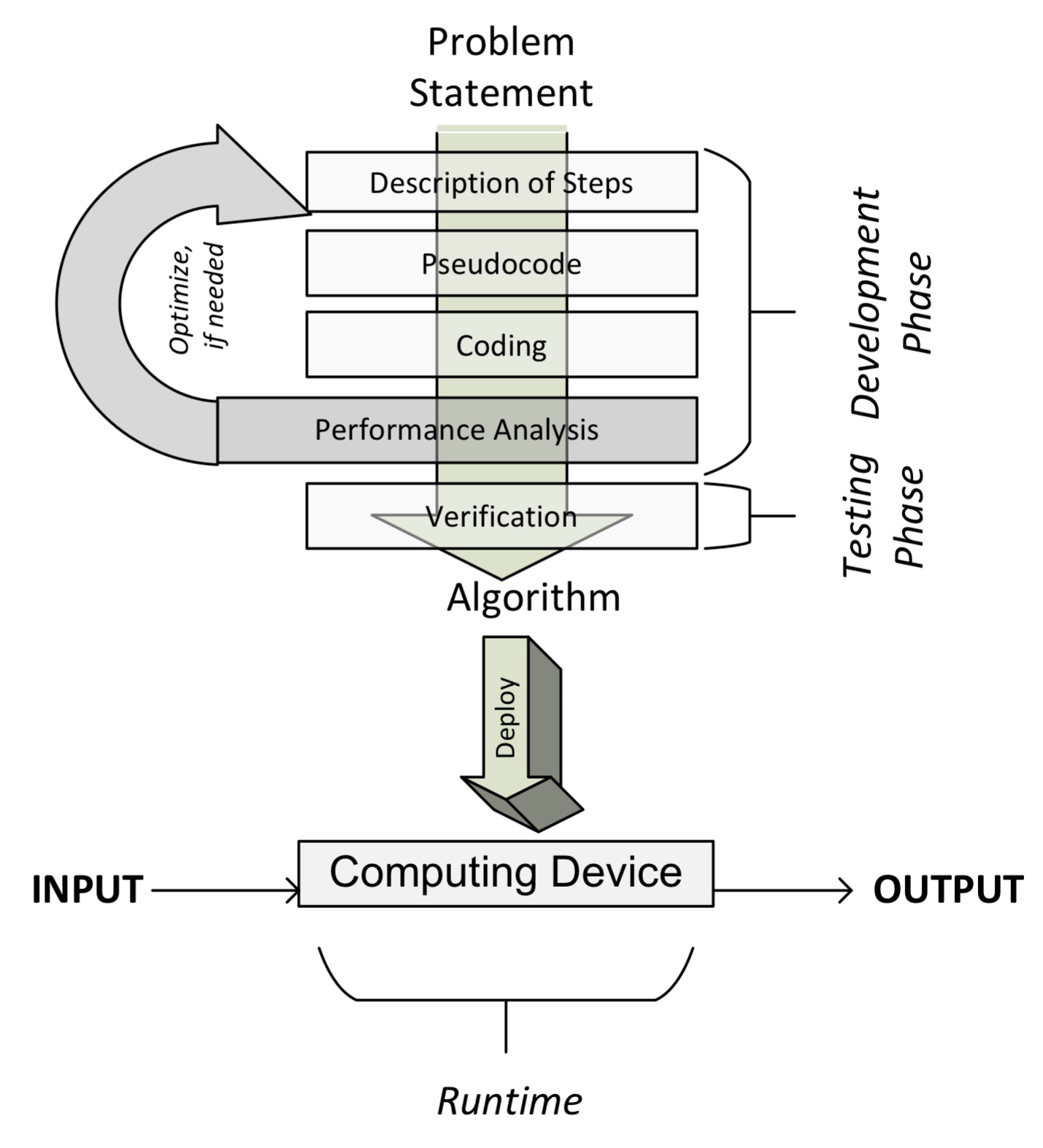
Analyzing the performance of an algorithm is an important part of its design. One of the ways to estimate the performance of an algorithm is to analyze its complexity.

Complexity theory is the study of how complicated algorithms are. To be useful, any algorithm should have three key features:

• It should be correct. An algorithm won't do you much good if it doesn't give you the right answers.

• A good algorithm should be understandable. The best algorithm in the world won't do you any good if it's too complicated for you to implement on a computer.

• A good algorithm should be efficient. Even if an algorithm produces a correct result, it won't help you much if it takes a thousand years or if it requires 1 billion terabytes of memory.

There are two possible types of analysis to quantify the complexity of an algorithm:

• Space complexity analysis: Estimates the runtime memory requirements needed to execute the algorithm.

• Time complexity analysis: Estimates the time the algorithm will take to run.

Space complexity analysis estimates the amount of memory required by the algorithm to process input data. While processing the input data, the algorithm needs to store the transient temporary data structures in memory. The way the algorithm is designed affects the number, type, and size of these data structures. In an age of distributed computing and with increasingly large amounts of data that needs to be processed, space complexity analysis is becoming more and more important. The size, type, and number of these data structures will dictate the memory requirements for the underlying hardware. Modern in-memory data structures used in distributed computing—such as Resilient Distributed Datasets (RDDs)—need to have efficient resource allocation mechanisms that are aware of the memory requirements at different execution phases of the algorithm.

Space complexity analysis is a must for the efficient design of algorithms. If proper space complexity analysis is not conducted while designing a particular algorithm, insufficient memory availability for the transient temporary data structures may trigger unnecessary disk spillovers, which could potentially considerably affect the performance and efficiency of the algorithm.

In this chapter, we will look deeper into time complexity. Space complexity will be discussed in Chapter 13, Large-Scale Algorithms, in more detail, where we will deal with large-scale distributed algorithms with complex runtime memory requirements.

Time complexity analysis estimates how long it will take for an algorithm to complete its assigned job based on its structure. In contrast to space complexity, time complexity is not dependent on any hardware that the algorithm will run on. Time complexity analysis solely depends on the structure of the algorithm itself. The overall goal of time complexity analysis is to try to answer these important questions—will this algorithm scale? How well will this algorithm handle larger datasets?

To answer these questions, we need to determine the effect on the performance of an algorithm as the size of the data is increased and make sure that the algorithm is designed in a way that not only makes it accurate but also scales well. The performance of an algorithm is becoming more and more important for larger datasets in today's world of "big data."

In many cases, we may have more than one approach available to design the algorithm. The goal of conducting time complexity analysis, in this case, will be as follows:

There can be two basic approaches to calculating the time complexity of an algorithm:

• A post-implementation profiling approach: In this approach, different candidate algorithms are implemented and their performance is compared. 

• A pre-implementation theoretical approach: In this approach, the performance of each algorithm is approximated mathematically before running an algorithm.

The advantage of the theoretical approach is that it only depends on the structure of the algorithm itself. It does not depend on the actual hardware that will be used to run the algorithm, the choice of the software stack chosen at runtime, or the programming language used to implement the algorithm.

The performance of a typical algorithm will depend on the type of the data given to it as an input. For example, if the data is already sorted according to the context of the problem we are trying to solve, the algorithm may perform blazingly fast. If the sorted input is used to benchmark this particular algorithm, then it will give an unrealistically good performance number, which will not be a true reflection of its real performance in most scenarios. To handle this dependency of algorithms on the input data, we have different types of cases to consider when conducting a performance analysis.

In the best case, the data given as input is organized in a way that the algorithm will give its best performance. Best-case analysis gives the upper bound of the performance.

The second way to estimate the performance of an algorithm is to try to find the maximum possible time it will take to get the job done under a given set of conditions. This worst-case analysis of an algorithm is quite useful as we are guaranteeing that regardless of the conditions, the performance of the algorithm will always be better than the numbers that come out of our analysis. Worst-case analysis is especially useful for estimating the performance when dealing with complex problems with larger datasets. Worst-case analysis gives the lower bound of the performance of the algorithm. 

 This starts by dividing the various possible inputs into various groups. Then, it conducts the performance analysis from one of the representative inputs from each group. Finally, it calculates the average of the performance of each of the groups. 

 Average-case analysis is not always accurate as it needs to consider all the different combinations and possibilities of input to the algorithm, which is not always easy to do.

How do you know which one is a better solution? How do you know which algorithm runs faster? Time complexity and Big O notation (discussed later in this chapter) are really good tools for answering these types of questions.

To see where it can be useful, let's take a simple example where the objective is to sort a list of numbers. There are a couple of algorithms available that can do the job. The issue is how to choose the right one.

First, an observation that can be made is that if there are not too many numbers in the list, then it does not matter which algorithm do we choose to sort the list of numbers. So, if there are only 10 numbers in the list (n=10), then it does not matter which algorithm we choose as it would probably not take more than a few microseconds, even with a very badly designed algorithm. But as soon as the size of the list becomes 1 million, now the choice of the right algorithm will make a difference. A very badly written algorithm might even take a couple of hours to run, while a well-designed algorithm may finish sorting the list in a couple of seconds. So, for larger input datasets, it makes a lot of sense to invest time and effort, perform a performance analysis, and choose the correctly designed algorithm that will do the job required in an efficient manner.

Big O notation is used to quantify the performance of various algorithms as the input size grows. Big O notation is one of the most popular methodologies used to conduct worst-case analysis. The different kinds of Big O notation types are discussed in this section.

If an algorithm takes the same amount of time to run, independent of the size of the input data, it is said to run in constant time. It is represented by O(1). Let's take the example of accessing the n^th element of an array. Regardless of the size of the array, it will take constant time to get the results. For example, the following function will return the first element of the array and has a complexity of O(1):

def getFirst(myList):
    return myList[0]

The output is shown as:

• Addition of a new element to a stack by using push or removing an element from a stack by using pop. Regardless of the size of the stack, it will take the same time to add or remove an element.

• Accessing the element of the hashtable (as discussed in Chapter 2, Data Structures Used in Algorithms).

• Bucket sort (as discussed in Chapter 2, Data Structures Used in Algorithms).

An algorithm is said to have a complexity of linear time, represented by O(n), if the execution time is directly proportional to the size of the input. A simple example is to add the elements in a single-dimensional data structure:

def getSum(myList):
    sum = 0
    for item in myList:
        sum = sum + item
    return sum

Note the main loop of the algorithm. The number of iterations in the main loop increases linearly with an increasing value of n, producing an O(n) complexity in the following figure:

Some other examples of array operations are as follows:

• Searching an element

• Finding the minimum value among all the elements of an array

An algorithm is said to run in quadratic time if the execution time of an algorithm is proportional to the square of the input size; for example, a simple function that sums up a two-dimensional array, as follows:

def getSum(myList):
    sum = 0
    for row in myList:
        for item in row:
            sum += item
    return sum

Note the nested inner loop within the other main loop. This nested loop gives the preceding code the complexity of O(n²):

Another example is the bubble sort algorithm (as discussed in Chapter 2, Data Structures Used in Algorithms).

An algorithm is said to run in logarithmic time if the execution time of the algorithm is proportional to the logarithm of the input size. With each iteration, the input size decreases by a constant multiple factor. An example of logarithmic is binary search. The binary search algorithm is used to find a particular element in a one-dimensional data structure, such as a Python list. The elements within the data structure need to be sorted in descending order. The binary search algorithm is implemented in a function named searchBinary, as follows:

def searchBinary(myList,item):
    first = 0
    last = len(myList)-1
    foundFlag = False
    while( first<=last and not foundFlag):
        mid = (first + last)//2
        if myList[mid] == item :
            foundFlag = True
        else:
            if item < myList[mid]:
                last = mid - 1
            else:
                first = mid + 1
    return foundFlag

The main loop takes advantage of the fact that the list is ordered. It divides the list in half with each iteration until it gets to the result:

After defining the function, it is tested to search a particular element in lines 11 and 12. The binary search algorithm is further discussed in Chapter 3, Sorting and Searching Algorithms.

Note that among the four types of Big O notation types presented, O(n²) has the worst performance and O(logn) has the best performance. In fact, O(logn)'s performance can be thought of as the gold standard for the performance of any algorithm (which is not always achieved, though). On the other hand, O(n²) is not as bad as O(n³) but still, algorithms that fall in this class cannot be used on big data as the time complexity puts limitations on how much data they can realistically process.

One way to reduce the complexity of an algorithm is to compromise on its accuracy, producing a type of algorithm called an approximate algorithm. 

The whole process of the performance evaluation of algorithms is iterative in nature, as shown in the following figure: