

While SmartList exports are great for sending Dynamics GP data to Excel for analysis, they aren't an ideal solution for a dashboard. SmartLists sends data to a new Excel file each time. It's a lot of work to export data and rebuild a dashboard every month. An improved option is to use a SmartList Export Solution.
SmartList Export Solutions let you export GP data to a saved Excel workbook. They also provide the option to run an Excel macro before and/or after the data populates in Excel. As an example, we will format the header automatically after exporting financial summary information.
We have a little setup work to do for this one first. Since these exports are typically repetitive, the setup is worth the effort. Here is how it's done:
Access SmartList in the same method used for SmartList exports (where you open SmartList depends on whether you are using the Rich Client or the Web Client of GP).
Go to
Financial|Account Summaryon the left-hand side to generate a SmartList.Click on the Excel button to send the SmartList to Excel.
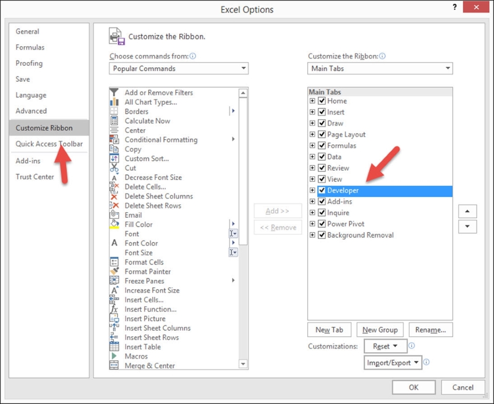
Next, we need to turn on Developer ribbon in Excel. In Excel 2016, go to File | Options | Customize Ribbon.
Select the box next to Developer on the right-hand side. Click on OK.
A SmartList Export Solution allows you to run an Excel macro before or after the data arrives to format or manipulate the information so that you only have to do it once. Let's record our Excel macro using these steps:
Click on the Developer tab and select Record Macro. Accept the default name of
Macro1and click on OK: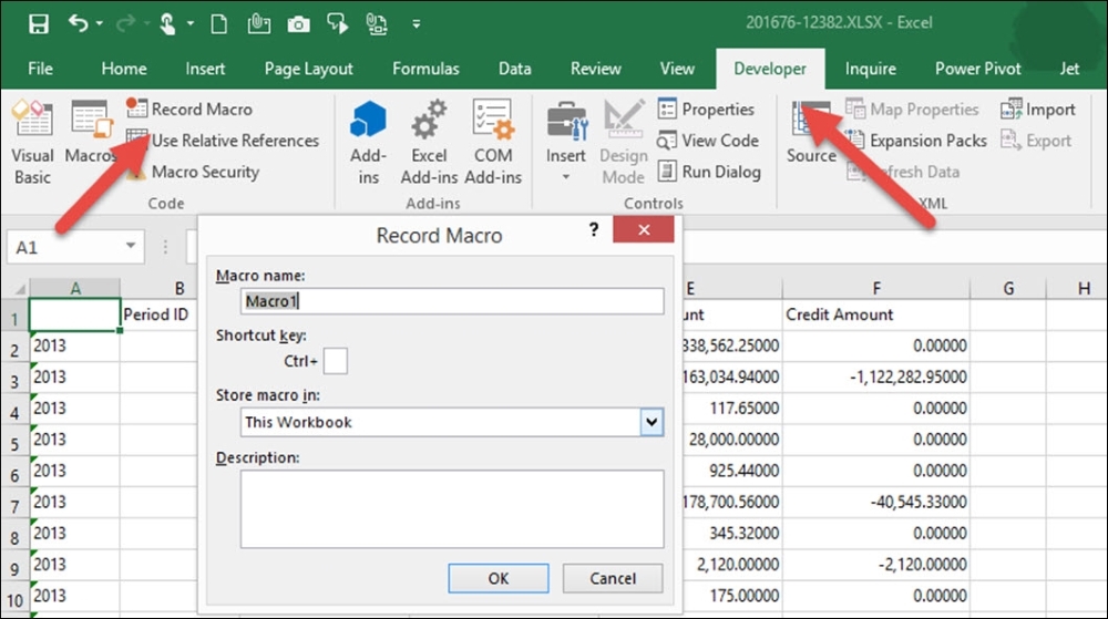
In Excel 2016, highlight rows 1-5, right-click, and select Insert.
Bold the titles in cells A6-F6 by highlighting them and clicking on the B icon on the Home ribbon.
In cell A1, enter
Sample Excel Solution.From the Developer tab, select Stop Recording.
Highlight and delete all the rows.
Save the blank file containing just the macro in
C:drive, with the name asAccountSummary.xlsm.
Now that we've prepared our Excel 2016 workbook to receive a SmartList, we need to set up and run the SmartList Export Solution using these steps:
Access SmartList in the same method used for SmartList exports (where you open SmartList depends on whether you are using the Rich Client or the Web Client of GP).
Go to
Financial|Account Summaryin the left pane to generate a SmartList.Click on Favorites. Go to Add | Add Favorite. The favorite can be named anything. I'm using
Export Solutionfor our example: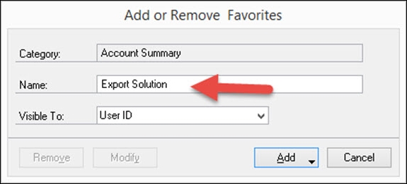
Back on the SmartList window, go to SmartList | Export Solutions. Name the solution
Export Solution. Set the path toC:\AccountSummary.xlsm(or where you saved your Excel file with the macro) and the completion macro toMacro1:
Select the box next to the SmartList favorite under
Account SummarynamedExport Solution:Make sure the Application is set to Excel. If not, change it:

Select Save and close the window.
Back in the SmartList window, select the
Export Solutionfavorite underAccount Summaryand click on the Excel button.Instead of immediately opening Excel, there are now two options. The Quick Export option performs a typical Excel export. We want the second option. Click on the Export Solution option. This will open the Excel file named
AccountSummary.xlsm, export the data, and run the macro namedMacro1, all with one click:
Click on the Export Solution option and watch the file open and the macro execute:

Without a doubt, this is a personal favorite method of getting GP data into Excel. "Why?" you ask. The reason is with Get and Transform you can:
Access your GP (SQL) data
Combine your GP data with non-GP data
Edit (or model) your GP data (by this, we mean you can combine fields, extract portions from fields, such as the year from a date, replace null values, and so on)
Merge or append tables together
And all of this can be done from within Excel without ever logging into a SQL tool such as the SQL Server Studio. You can have developer results while thinking like an Excel user and without being a developer.
Tip
There is a big advantage to learning this tool. It is the same tool that is used in Microsoft Power BI. So, learning this one tool in Excel gives you a huge advantage in Power BI.
In Excel 2013 and Excel 2010, this feature can be installed as an add-on called Power Query. Note that this feature only works on specific versions of Excel, so check the system requirements before downloading.
Tip
A table is a file that holds a set of records in the SQL Server. Imagine your chart of accounts being stored in an Excel spreadsheet, which could be a single table for some applications. However, many complex applications (such as Dynamics GP) often break up the information across several tables for efficiency. GP separates the chart of accounts into seven separate tables. Separating the data is good for the application, but confusing to non-developers or database administrators who just want a good Excel report.
To make it easier for users, often these virtual tables are created for the purpose of reporting to combine the data together and making the field names logical. A view is what a virtual table in the SQL Server is called. The chart of accounts information in GP, for example, can be found in an out-of-the-box view called Accounts.
Let's extract our list of General Ledger Accounts. Fortunately, Microsoft has already created this as a view in the SQL Database. This view has a lot of fields in it, but let's assume we want to make sure all of the accounts are set up with the correct type (Balance Sheet or Profit and Loss) so that when we close the year in the General Ledger, only the Balance Sheet accounts will roll forward into the new year. Follow these steps:
Open Microsoft Excel 2016.
Go to Data | New Query | From Database | From SQL Server Database:
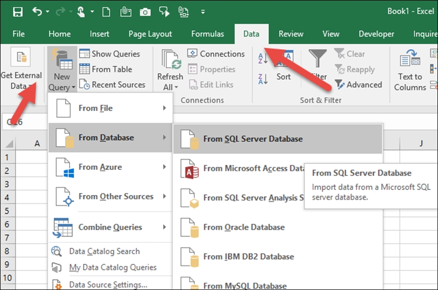
In the SQL Server Database window that appears, enter the name of your SQL Server instance in the Server and Database (optional) field. Our GP data is located on the server named
Cherryand the Database isTWO. Click on OK: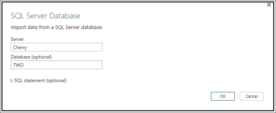
The Navigator window will open, displaying all the tables and views in the SQL Database you selected. Highlight the
Accountsview on the left-hand side. You will then get a preview of this view on the right-hand side. Click on Edit: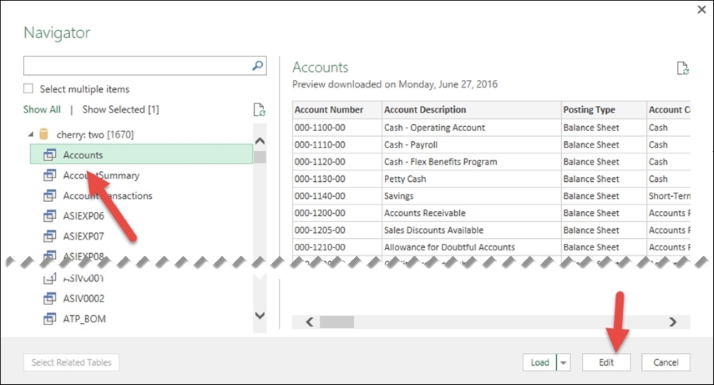
The Query Editor window will open with the
Accountsdata loaded. The first step should always be to rename this query to something that represents something that makes sense to the consumer of this report. We will rename ours toChart of Accounts: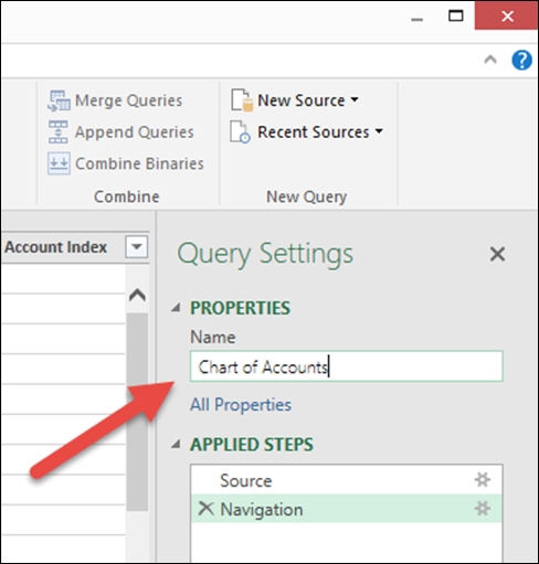
Click on the Table icon and select Choose Columns:
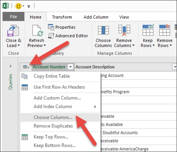
The Choose Columns window will open. Unmark the first item in the list titled (Select All Columns) so that we can manually select the ones we want to keep. Select Account Number, Account Description, Posting Type, Account Type, Active, and Created Date. Click on OK. Now, only the columns selected are displayed:

The second-most important step is verifying that the column data type is correct. Highlight the Account Number column, hold the Shift key down, and select the Active column so that all columns are highlighted. Right-click on the highlighted area and go to Change Type | Text. It might already be Text, but this just confirms. You can also highlight the columns one at a time and check the Data Type in the ribbon.
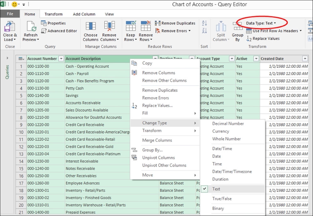
Highlight the last column, Created Date, right-click and go to Change Type | Date. This will change the date format from one that displays the time to one that displays only the date:
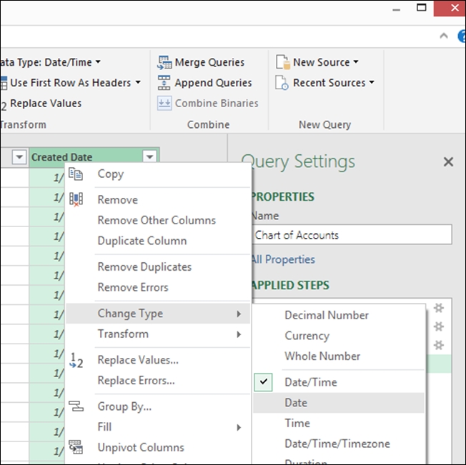
You'll notice that as we perform each step, our actions are recorded in the Applied Steps area. Get and Transform is actually recording everything we do, so when we use this query again, all of the steps will automatically be performed for us:

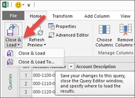
Each column has a filter, so you can choose to filter the data if you desire. Click on the words where the down arrow is located (not the icon) for Close & Load | Close & Load To… If we click on the icon, the data will flow into a table in Excel. Using the Close & Load To… feature, we can load the data into the Excel in-memory data model (Power Pivot):
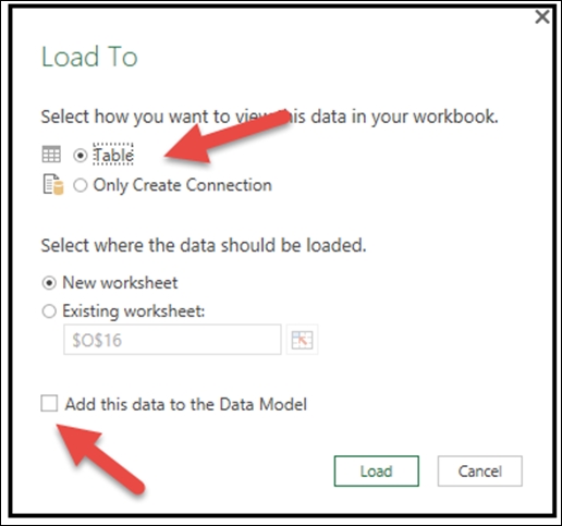
The Load To window opens. From here, you can either load the data to a table in the worksheet or create the connection only that would allow you to save the Excel file without the data. This allows you to refresh the data without saving a large file (but you must be connected to the SQL Server for this to refresh). You can also choose to add the data to the data model. The data is attached to the Excel file, but not visible to the spreadsheet. This is a great option if you only plan to create a PivotTable. Click on Load:
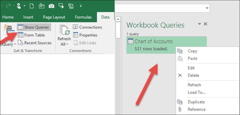
You'll notice there is a Workbook Queries pane whose display can be turned on or off using the Show Queries option on the Data ribbon. Right-clicking on the query provides you with many options, including the ability to Edit the query:
This is only a tiny fraction of what Get and Transform can do. You'll learn more about this great feature in Chapter 12, Sharing and Refreshing Data and Dashboards in Power BI.