
An important class of linear time series models is the family of Autoregressive Integrated Moving Average (ARIMA) models, proposed by Box and Jenkins (1976). It assumes that the current value can depend only on the past values of the time series itself or on past values of some error term.
According to Box and Jenkins, building an ARIMA model consists of three stages:
Model identification.
Model estimation.
Model diagnostic checking.
The model identification step involves determining the order (number of past values and number of past error terms to incorporate) of a tentative model using either graphical methods or information criteria. After determining the order of the model, the parameters of the model need to be estimated, generally using either the least squares or maximum likelihood methods. The fitted model must then be carefully examined to check for possible model inadequacies. This is done by making sure the model residuals behave as white noise; that is, there is no linear dependence left in the residuals.
In addition to the zoo package, we will employ some methods from the forecast package. If you haven't installed it already, you need to use the following command to do so:
> install.packages("forecast")
Afterwards, we need to load the class using the following command:
> library("forecast")
First, we store the monthly house price data (source: Nationwide Building Society) in a zoo time series object.
> hp <- read.zoo("UKHP.csv", sep = ",",+ header = TRUE, format = "%Y-%m", FUN = as.yearmon)
The FUN argument applies the given function (as.yearmon, which represents the monthly data points) to the date column. To make sure we really stored monthly data (12 subperiods per period), by specifying as.yearmon, we query for the frequency of the data series.
> frequency(hp)
[1] 12
The result means that we have twelve subperiods (called months) in a period (called year). We again use simple returns for our analysis.
> hp_ret <- diff(hp) / lag(hp, k = -1) * 100
We use the auto.arima function provided by the forecast package to identify the optimal model and estimate the coefficients in one step. The function takes several arguments besides the return series (hp_ret). By specifying stationary = TRUE,we restrict the search to stationary models. In a similar vein, seasonal = FALSE restricts the search to non-seasonal models. Furthermore, we select the Akaike information criteria as the measure of relative quality to be used in model selection.
> mod <- auto.arima(hp_ret, stationary = TRUE, seasonal = FALSE,+ ic="aic")
To determine the fitted coefficient values, we query the model output.
> mod
Series: hp_ret
ARIMA(2,0,0) with non-zero mean

Coefficients:
         ar1     ar2  intercept
      0.2299  0.3491     0.4345
s.e.  0.0573  0.0575     0.1519

sigma^2 estimated as 1.105:  log likelihood=-390.97
AIC=789.94   AICc=790.1   BIC=804.28
An AR(2) process seems to fit the data best, according to Akaike's Information Criteria. For visual confirmation, we can plot the partial autocorrelation function using the command pacf. It shows non-zero partial autocorrelations until lag two, hence an AR process of order two seems to be appropriate. The two AR coefficients, the intercept (which is actually the mean if the model contains an AR term), and the respective standard errors are given. In the following example, they are all significant at the 5% level since the respective confidence intervals do not contain zero:
> confint(mod)
              2.5 %    97.5 %
ar1       0.1174881 0.3422486
ar2       0.2364347 0.4617421
intercept 0.1368785 0.7321623
If the model contains coefficients that are insignificant, we can estimate the model anew using the arima function with the fixed argument, which takes as input a vector of elements 0 and NA. NA indicates that the respective coefficient shall be estimated and 0 indicates that the respective coefficient should be set to zero.
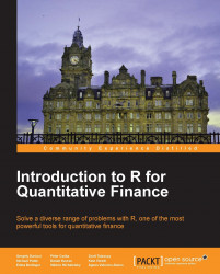
A quick way to validate the model is to plot time-series diagnostics using the following command:
> tsdiag(mod)
The output of the preceding command is shown in the following figure:
Our model looks good since the standardized residuals don't show volatility clusters, no significant autocorrelations between the residuals according to the ACF plot, and the Ljung-Box test for autocorrelation shows high p-values, so the null hypothesis of independent residuals cannot be rejected.
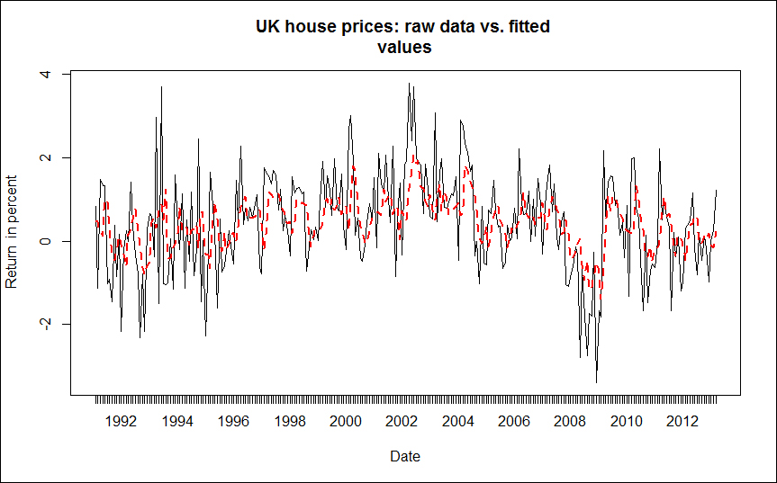
To assess how well the model represents the data in the sample, we can plot the raw monthly returns (the thin black solid line) versus the fitted values (the thick red dotted line).
> plot(mod$x, lty = 1, main = "UK house prices: raw data vs. fitted+   values", ylab = "Return in percent", xlab = "Date")
> lines(fitted(mod), lty = 2,lwd = 2, col = "red")
The output is shown in the following figure:
Furthermore, we can calculate common measures of accuracy.
> accuracy(mod)
ME      RMSE      MAE          MPE   MAPE    MASE
0.00120 1.0514    0.8059       -Inf  Inf     0.792980241
This command returns the mean error, root mean squared error, mean absolute error, mean percentage error, mean absolute percentage error, and mean absolute scaled error.
To predict the monthly returns for the next three months (April to June 2013), use the following command:
> predict(mod, n.ahead=3)
$pred
           Apr       May       Jun
2013 0.5490544 0.7367277 0.5439708

$se
          Apr      May      Jun
2013 1.051422 1.078842 1.158658
So we expect a slight increase in the average home prices over the next three months, but with a high standard error of around 1%. To plot the forecast with standard errors, we can use the following command:
> plot(forecast(mod))