Book Image

Introduction to R for Quantitative Finance

Book Image

Introduction to R for Quantitative Finance

Overview of this book

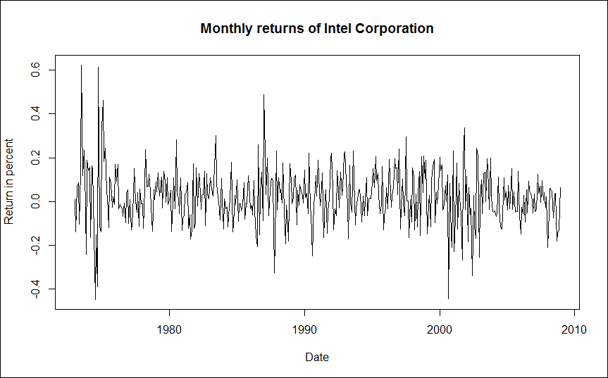
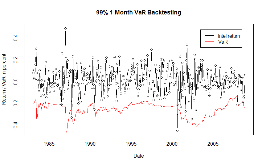
Introduction to R for Quantitative Finance will show you how to solve real-world quantitative fi nance problems using the statistical computing language R. The book covers diverse topics ranging from time series analysis to fi nancial networks. Each chapter briefl y presents the theory behind specific concepts and deals with solving a diverse range of problems using R with the help of practical examples.This book will be your guide on how to use and master R in order to solve quantitative finance problems. This book covers the essentials of quantitative finance, taking you through a number of clear and practical examples in R that will not only help you to understand the theory, but how to effectively deal with your own real-life problems.Starting with time series analysis, you will also learn how to optimize portfolios and how asset pricing models work. The book then covers fixed income securities and derivatives such as credit risk management.
Table of Contents (17 chapters)
Introduction to R for Quantitative Finance
Credits
About the Authors
About the Reviewers
www.PacktPub.com
Preface
Index

Modeling volatility


As we saw earlier, ARIMA models are used to model the conditional expectation of a process, given its past. For such a process, the conditional variance is constant. Real-world financial time series exhibit, among other characteristics, volatility clustering; that is, periods of relative calm are interrupted by bursts of volatility.

In this section we look at GARCH time series models that can take this stylized fact of real-world (financial) time series into account and apply these models to VaR forecasting.

Volatility forecasting for risk management

Financial institutions measure the risk of their activities using a Value-at-Risk (VaR), usually calculated at the 99% confidence level over a 10 business day horizon. This is the loss that is expected to be exceeded only 1% of the time.

We load the zoo library and import monthly return data for Intel Corporation from January 1973 to December 2008.

> library("zoo")
> intc <- read.zoo("intc.csv", header = TRUE,+   sep = ",", format = "%Y-%m", FUN = as.yearmon)

Testing for ARCH effects

A plot of the returns indicates that ARCH effects might exist in the monthly return data.

> plot(intc, main = "Monthly returns of Intel Corporation",+   xlab = "Date", ylab = "Return in percent")

The output of the preceding commands is as shown in the following figure:

We can use statistical hypothesis tests to verify our inkling. Two commonly used tests are as follows:

  • The Ljung-Box test for autocorrelation in squared returns (as a proxy for volatility)

  • The Lagrange Multiplier (LM) test by Engle (1982)

First, we perform the Ljung-Box test on the first 12 lags of the squared returns using the following command:

> Box.test(coredata(intc^2), type = "Ljung-Box", lag = 12)

   Box-Ljung test

data:  coredata(intc^2)
X-squared = 79.3451, df = 12, p-value = 5.502e-12

We can reject the null hypothesis of no autocorrelations in the squared returns at the 1% significance level. Alternatively, we could employ the LM test from the FinTS package, which gives the same result.

> install.packages("FinTS")
> library("FinTS")
> ArchTest(coredata(intc))

   ARCH LM-test; Null hypothesis: no ARCH effects

data:  coredata(intc)
Chi-squared = 59.3647, df = 12, p-value = 2.946e-08

Both tests confirm that ARCH effects exist in the monthly Intel returns; hence, an ARCH or GARCH model should be employed in modeling the return time series.

GARCH model specification

The most commonly used GARCH model, and one that is usually appropriate for financial time series as well, is a GARCH(1,1) model. We use the functions provided by the rugarch library for model specification, parameter estimation, backtesting, and forecasting. If you haven't installed the package, use the following command:

> install.packages("rugarch")

Afterwards, we can load the library using the following command:

> library("rugarch")

First, we need to specify the model using the function ugarchspec. For a GARCH(1,1) model, we need to set the garchOrder to c(1,1) and the model for the mean (mean.model) should be a white noise process and hence equal to armaOrder = c(0,0).

> intc_garch11_spec <- ugarchspec(variance.model = list(+   garchOrder = c(1, 1)),+  mean.model = list(armaOrder = c(0, 0)))

GARCH model estimation

The actual fitting of the coefficients by the method of maximum likelihood is done by the function ugarchfit using the model specification and the return data as inputs.

> intc_garch11_fit <- ugarchfit(spec = intc_garch11_spec,+  data = intc)

For additional arguments, see the Help on ugarchfit. The output of the fitted model (use the command intc_garch11_fit) reveals useful information, such as the values of the optimal parameters, the value of the log-likelihood function, and the information criteria.

Backtesting the risk model

A useful test for checking the model performance is to do a historical backtest. In a risk model backtest, we compare the estimated VaR with the actual return over the period. If the return is more negative than the VaR, we have a VaR exceedance. In our case, a VaR exceedance should only occur in 1% of the cases (since we specified a 99% confidence level).

The function ugarchroll performs a historical backtest on the specified GARCH model (here the model is intc_garch11_spec). We specify the backtest as follows:

  • The return data to be used is stored in the zoo object intc

  • The start period of the backtest (n.start) shall be 120 months after the beginning of the series (that is, January 1983)

  • The model should be reestimated every month (refit.every = 1)

  • We use a moving window for the estimation

  • We use a hybrid solver

  • We'd like to calculate the VaR (calculate.VaR = TRUE) at the 99% VaR tail level (VaR.alpha = 0.01)

  • We would like to keep the estimated coefficients (keep.coef = TRUE)

The following command shows all the preceding points for a backtest:

> intc_garch11_roll <- ugarchroll(intc_garch11_spec, intc,+   n.start = 120, refit.every = 1, refit.window = "moving",+   solver = "hybrid", calculate.VaR = TRUE, VaR.alpha = 0.01,+   keep.coef = TRUE)

We can examine the backtesting report using the report function. By specifying the type argument as VaR, the function executes the unconditional and conditional coverage tests for exceedances. VaR.alpha is the tail probability and conf.level is the confidence level on which the conditional coverage hypothesis test will be based.

> report(intc_garch11_roll, type = "VaR", VaR.alpha = 0.01,+   conf.level = 0.99)
VaR Backtest Report
===========================================
Model:            sGARCH-norm
Backtest Length:   312
Data:            

==========================================
alpha:            1%
Expected Exceed:   3.1
Actual VaR Exceed:	5
Actual %:         1.6%

Unconditional Coverage (Kupiec)
Null-Hypothesis:   Correct Exceedances
LR.uc Statistic:   0.968
LR.uc Critical:      6.635
LR.uc p-value:      0.325
Reject Null:      NO

Conditional Coverage (Christoffersen)
Null-Hypothesis:   Correct Exceedances and
               Independence of Failures
LR.cc Statistic:   1.131
LR.cc Critical:      9.21
LR.cc p-value:      0.568
Reject Null:      O

Kupiec's unconditional coverage compares the number of expected versus actual exceedances given the tail probability of VaR, while the Christoffersen test is a joint test of the unconditional coverage and the independence of the exceedances. In our case, despite the actual five exceedances versus an expectation of three, we can't reject the null hypothesis that the exceedances are correct and independent.

A plot of the backtesting performance can also be generated easily. First, create a zoo object using the extracted forecasted VaR from the ugarchroll object.

> intc_VaR <- zoo(intc_garch11_roll@forecast$VaR[, 1])

We overwrite the index property of the zoo object with rownames (year and month) from this object as well.

> index(intc_VaR) <- as.yearmon(rownames(intc_garch11_roll@forecast$VaR))

We do the same for the actual returns that are also stored in the ugarchroll object.

> intc_actual <- zoo(intc_garch11_roll@forecast$VaR[, 2])
> index(intc_actual) <- as.yearmon(rownames(intc_garch11_roll@forecast$VaR))

Now, we are able to plot the VaR versus the actual returns of Intel using the following commands:

> plot(intc_actual, type = "b", main = "99% 1 Month VaR Backtesting",+   xlab = "Date", ylab = "Return/VaR in percent")
> lines(intc_VaR, col = "red")
> legend("topright", inset=.05, c("Intel return","VaR"), col = c("black","red"), lty = c(1,1))

The following figure shows the output of the preceding command lines:

Forecasting

Now that we can be reasonably sure that our risk model works properly, we can produce VaR forecasts as well. The function ugarchforecast takes as arguments the fitted GARCH model (intc_garch11_fit) and the number of periods for which a forecast should be produced (n.ahead = 12; that is, twelve months).

> intc_garch11_fcst <- ugarchforecast(intc_garch11_fit, n.ahead = 12)

The resulting forecast can be expected by querying the forecast object as shown in the following command lines:

> intc_garch11_fcst
*------------------------------------*
*       GARCH Model Forecast         *
*------------------------------------*
Model: sGARCH
Horizon: 12
Roll Steps: 0
Out of Sample: 0

0-roll forecast [T0=Dec 2008]:
      Series  Sigma
T+1  0.01911 0.1168
T+2  0.01911 0.1172
T+3  0.01911 0.1177
T+4  0.01911 0.1181
T+5  0.01911 0.1184
T+6  0.01911 0.1188
T+7  0.01911 0.1191
T+8  0.01911 0.1194
T+9  0.01911 0.1197
T+10 0.01911 0.1200
T+11 0.01911 0.1202
T+12 0.01911 0.1204

The one-period ahead forecast for the volatility (sigma) is 0.1168. Since we assume a normal distribution, the 99% VaR can be calculated using the 99% quantile (type in qnorm(0.99)) of the standard normal distribution. The one-month 99% VaR estimate for the next period is hence qnorm(0.99)*0.1168 = 0.2717. Hence, with 99% probability the monthly return is above -27%.