As we saw in the previous sections, this main target audience of the book is developers who want to understand machine learning algorithms. But in order to really grasp the motivations and reason behind them, it's necessary to review and build all the fundamental reasoning, which includes statistics, probability, and calculus.

We will first start with some of the fundamentals of statistics.

Statistics can be defined as a discipline that uses data samples to extract and support conclusions about larger samples of data. Given that machine learning comprises a big part of the study of the properties of data and the assignment of values to data, we will use many statistical concepts to define and justify the different methods.

In the following sections, we will start defining the fundamental operations and measures of the discipline of statistics in order to be able to advance from the fundamental concepts.

This is one of the most intuitive and most frequently used concepts in statistics. Given a set of numbers, the mean of that set is the sum of all the elements divided by the number of elements in the set.

The formula that represents the mean is as follows:

Although this is a very simple concept, we will write a Python code sample in which we will create a sample set, represent it as a line plot, and mark the mean of the whole set as a line, which should be at the weighted center of the samples. It will serve as an introduction to Python syntax, and also as a way of experimenting with Jupyter notebooks:

    import matplotlib.pyplot as plt #Import the plot library 
 
    def mean(sampleset):  #Definition header for the mean function 
        total=0 
        for element in sampleset: 
            total=total+element 
        return total/len(sampleset) 
 
    myset=[2.,10.,3.,6.,4.,6.,10.]  #We create the data set 
    mymean=mean(myset) #Call the mean funcion 
    plt.plot(myset)  #Plot the dataset 
    plt.plot([mymean] * 7)  #Plot a line of 7 points located on the mean 

This program will output a time series of the dataset elements, and will then draw a line at the mean height.

As the following graph shows, the mean is a succinct (one value) way of describing the tendency of a sample set:

In this first example, we worked with a very homogeneous sample set, so the mean is very informative regarding its values. But let's try the same sample with a very dispersed sample set (you are encouraged to play with the values too):

As we saw in the first example, the mean isn't sufficient to describe non-homogeneous or very dispersed samples.

In order to add a unique value describing how dispersed the sample set's values are, we need to look at the concept of variance, which needs the mean of the sample set as a starting point, and then averages the distances of the samples from the provided mean. The greater the variance, the more scattered the sample set.

The canonical definition of variance is as follows:

Let's write the following sample code snippet to illustrate this concept, adopting the previously used libraries. For the sake of clarity, we are repeating the declaration of the mean function:

    import math #This library is needed for the power operation 
    def mean(sampleset):  #Definition header for the mean function 
        total=0 
        for element in sampleset: 
            total=total+element 
        return total/len(sampleset) 
 
    def variance(sampleset):  #Definition header for the mean function 
        total=0 
        setmean=mean(sampleset) 
        for element in sampleset: 
            total=total+(math.pow(element-setmean,2)) 
        return total/len(sampleset) 
 
    myset1=[2.,10.,3.,6.,4.,6.,10.]  #We create the data set 
    myset2=[1.,-100.,15.,-100.,21.] 
    print "Variance of first set:" + str(variance(myset1)) 
    print "Variance of second set:" + str(variance(myset2)) 
 

The preceding code will generate the following output:

    Variance of first set:8.69387755102
    Variance of second set:3070.64

As you can see, the variance of the second set was much higher, given the really dispersed values. The fact that we are computing the mean of the squared distance helps to really outline the differences, as it is a quadratic operation.

Standard deviation is simply a means of regularizing the square nature of the mean square used in the variance, effectively linearizing this term. This measure can be useful for other, more complex operations.

Here is the official form of standard deviation:

We are now about to study the single most important discipline required for understanding all the concepts of this book.

Probability is a mathematical discipline, and its main occupation is the study of random events. In a more practical definition, probability normally tries to quantify the level of certainty (or conversely, uncertainty) associated with an event, from a universe of possible occurrences.

In order to understand probabilities, we first need to define events. An event is, given an experiment in which we perform a determined action with different possible results, a subset of all the possible outcomes for that experiment.

Examples of events are a particular dice number appearing, and a product defect of particular type appearing on an assembly line.

Following the previous definitions, probability is the likelihood of the occurrence of an event. Probability is quantified as a real number between 0 and 1, and the assigned probability P increases towards 1 when the likelihood of the event occurring increases.

The mathematical expression for the probability of the occurrence of an event is P(E).

When assigning event probabilities, we could also try to cover the entire sample and assign one probability value to each of the possible outcomes for the sample domain.

This process does indeed have all the characteristics of a function, and thus we will have a random variable that will have a value for each one of the possible event outcomes. We will call this function a random function.

These variables can be of the following two types:

• Discrete: If the number of outcomes is finite, or countably infinite
• Continuous: If the outcome set belongs to a continuous interval

This probability function is also called probability distribution.

Between the multiple possible probability distributions, there are a number of functions that have been studied and analyzed for their special properties, or the popular problems they represent.

We will describe the most common ones that have a special effect on the development of machine learning.

Let's begin with a simple distribution: one that has a binary outcome, and is very much like tossing a (fair) coin.

This distribution represents a single event that takes the value 1 (let's call this heads) with a probability of p, and 0 (lets call this tails), with probability 1-p.

In order to visualize this, let's generate a large number of events of a Bernoulli distribution using np and graph the tendency of this distribution, with the following only two possible outcomes:

    plt.figure() 
    distro = np.random.binomial(1, .6, 10000)/0.5 
    plt.hist(distro, 2 , normed=1) 

The following graph shows the binomial distribution, through an histogram, showing the complementary nature of the outcomes' probabilities:

So, here we see the very clear tendency of the complementing probabilities of the possible outcomes. Now let's complement the model with a larger number of possible outcomes. When their number is greater than 2, we are talking about a multinomial distribution:

    plt.figure()
    distro = np.random.binomial(100, .6, 10000)/0.01 
    plt.hist(distro, 100 , normed=1) 
    plt.show() 

Take a look at the following graph:

This very common distribution is the first continuous distribution that we will see. As the name implies, it has a constant probability value for any interval of the domain.

In order to integrate to 1, a and b being the extreme of the function, this probability has the value of 1/(b-a).

Let's generate a plot with a sample uniform distribution using a very regular histogram, as generated by the following code:

    plt.figure() 
    uniform_low=0.25 
    uniform_high=0.8 
                         
    plt.hist(uniform, 50, normed=1) 
    plt.show() 

Take look at the following graph:

This very common continuous random function, also called a Gaussian function, can be defined with the simple metrics of the mean and the variance, although in a somewhat complex form.

This is the canonical form of the function:

Take a look at the following code snippet:

    import matplotlib.pyplot as plt #Import the plot library 
    import numpy as np 
    mu=0. 
    sigma=2. 
    distro = np.random.normal(mu, sigma, 10000) 
    plt.hist(distro, 100, normed=True) 
    plt.show() 

The following graph shows the generated distribution's histogram:

This distribution is similar to the normal distribution, but with the morphological difference of having a more elongated tail. The main importance of this distribution lies in its cumulative distribution function (CDF), which we will be using in the following chapters, and will certainly look familiar.

Let's first represent the base distribution by using the following code snippet:

    import matplotlib.pyplot as plt #Import the plot library 
    import numpy as np 
    mu=0.5 
    sigma=0.5 
    distro2 = np.random.logistic(mu, sigma, 10000) 
    plt.hist(distro2, 50, normed=True) 
    distro = np.random.normal(mu, sigma, 10000) 
    plt.hist(distro, 50, normed=True) 
    plt.show() 

Take a look at the following graph:

Then, as mentioned before, let's compute the CDF of the logistic distribution so that you will see a very familiar figure, the sigmoid curve, which we will see again when we review neural network activation functions:

    plt.figure() 
    logistic_cumulative = np.random.logistic(mu, sigma, 10000)/0.02 
    plt.hist(logistic_cumulative, 50, normed=1, cumulative=True) 
    plt.show() 

Take a look at the following graph:

In this section, we will see the most common statistical measures that can be applied to probabilities. The first measures are the mean and variance, which do not differ from the definitions we saw in the introduction to statistics.

This measure represents the lateral deviation, or in general terms, the deviation from the center, or the symmetry (or lack thereof) of a probability distribution. In general, if skewness is negative, it implies a deviation to the right, and if it is positive, it implies a deviation to the left:

Take a look at the following diagram, which depicts the skewness statistical distribution:

Kurtosis gives us an idea of the central concentration of a distribution, defining how acute the central area is, or the reverse—how distributed the function's tail is.

The formula for kurtosis is as follows:

In the following diagram, we can clearly see how the new metrics that we are learning can be intuitively understood:

To cover the minimum basic knowledge of machine learning, especially the learning algorithms such as gradient descent, we will introduce you to the concepts involved in differential calculus.

Covering the calculus terminology necessary to get to gradient descent theory would take many chapters, so we will assume you have an understanding of the concepts of the properties of the most well-known continuous functions, such as linear, quadratic, logarithmic, and exponential, and the concept of limit.

For the sake of clarity, we will develop the concept of the functions of one variable, and then expand briefly to cover multivariate functions.

We established the concept of functions in the previous section. With the exception of constant functions defined in the entire domain, all functions have some sort of value dynamics. That means that f(x1) is different than f(x2) for some determined values of x.

The purpose of differential calculus is to measure change. For this specific task, many mathematicians of the 17th century (Leibniz and Newton were the most prominent exponents) worked hard to find a simple model to measure and predict how a symbolically defined function changed over time.

This research guided the field to one wonderful concept—a symbolic result that, under certain conditions, tells you how much and in which direction a function changes at a certain point. This is the concept of a derivative.

If we want to measure how a function changes over time, the first intuitive step would be to take the value of a function and then measure it at the subsequent point. Subtracting the second value from the first would give us an idea of how much the function changes over time:

    import matplotlib.pyplot as plt 
    import numpy as np 
     %matplotlib inline 
 
    def quadratic(var): 
        return 2* pow(var,2) 
    x=np.arange(0,.5,.1) 
    plt.plot(x,quadratic(x)) 
    plt.plot([1,4], [quadratic(1), quadratic(4)],  linewidth=2.0) 
    plt.plot([1,4], [quadratic(1), quadratic(1)],  linewidth=3.0, 
    label="Change in x") 
    plt.plot([4,4], [quadratic(1), quadratic(4)],  linewidth=3.0, 
    label="Change in y") 
    plt.legend() 
    plt.plot (x, 10*x -8 ) 
    plt.plot() 

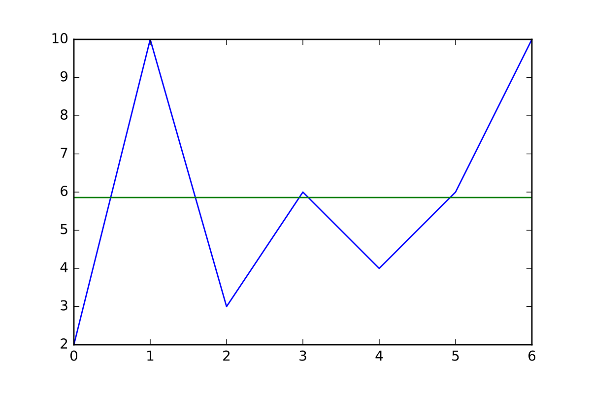
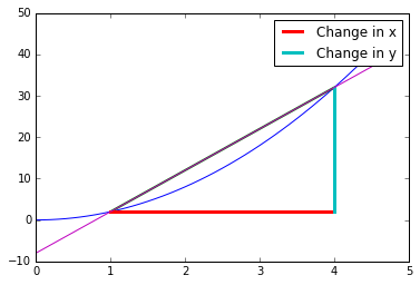
In the preceding code example, we first defined a sample quadratic equation (2*x²) and then defined the part of the domain in which we will work with the arange function (from 0 to 0.5, in 0.1 steps).

Then, we define an interval for which we measure the change of y over x, and draw lines indicating this measurement, as shown in the following graph:

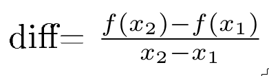
In this case, we measure the function at x=1 and x=4, and define the rate of change for this interval as follows:

Applying the formula, the result for the sample is (36-0)/3= 12.

This initial approach can serve as a way of approximately measuring this dynamic, but it's too dependent on the points at which we take the measurement, and it has to be taken at every interval we need.

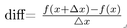
To have a better idea of the dynamics of a function, we need to be able to define and measure the instantaneous change rate at every point in the function's domain.

This idea of instantaneous change brings to us the need to reduce the distance between the domain's x values, taken at a point where there are very short distances between them. We will formulate this approach with an initial value x, and the subsequent value, x + Δx:

In the following code, we approximate the difference, reducing Δx progressively:

    initial_delta = .1 
    x1 = 1  
    for power in range (1,6): 
        delta = pow (initial_delta, power) 
        derivative_aprox= (quadratic(x1+delta) - quadratic (x1) )/ 
        ((x1+delta) - x1 ) 
        print "del    ta: " + str(delta) + ", estimated derivative: " + 
        str(derivative_aprox)  

In the preceding code, we first defined an initial delta, which brought an initial approximation. Then, we apply the difference function, with diminishing values of delta, thanks us to powering 0.1 with incremental powers. The results we get are as follows:

    delta: 0.1, estimated derivative: 4.2 
    delta: 0.01, estimated derivative: 4.02 
    delta: 0.001, estimated derivative: 4.002 
    delta: 0.0001, estimated derivative: 4.0002 
    delta: 1e-05, estimated derivative: 4.00002 

As the separation diminishes, it becomes clear that the change rate will hover around 4. But when does this process stop? In fact, we could say that this process can be followed ad infinitum, at least in a numeric sense.

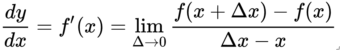
This is when the concept of limit intuitively appears. We will then define this process, of making Δ indefinitely smaller, and will call it the derivative of f(x) or f'(x):

This is the formal definition of the derivative.

But mathematicians didn't stop with these tedious calculations, making a large number of numerical operations (which were mostly done manually of the 17th century), and wanted to further simplify these operations.

What if we perform another step that can symbolically define the derivative of a function?

That would require building a function that gives us the derivative of the corresponding function, just by replacing the x variable value. That huge step was also reached in the 17th century, for different function families, starting with the parabolas (y=x²+b), and following with more complex functions:

One very important result of the symbolic determination of a function's derivative is the chain rule. This formula, first mentioned in a paper by Leibniz in 1676, made it possible to solve the derivatives of composite functions in a very simple and elegant manner, simplifying the solution for very complex functions.

In order to define the chain rule, if we suppose a function f, which is defined as a function of another function g, f(g(x)) of F, the derivative can be defined as follows:

The formula of the chain rule allows us to differentiate formulas whose input values depend on another function. This is the same as searching the rate of change of a function that is linked to a previous one. The chain rule is one of the main theoretical concepts employed in the training phase of neural networks, because in those layered structures, the output of the first neuron layers will be the inputs of the following, giving, as a result, a composite function that, most of the time, is of more than one nesting level.

Until now we've been working with univariate functions, but the type of function we will mostly work with from now on will be multivariate, as the dataset will contain much more than one column and each one of them will represent a different variable.

In many cases, we will need to know how the function changes in a relationship with only one dimension, which will involve looking at how one column of the dataset contributes to the total number of function changes.

The calculation of partial derivatives consists of applying the already known derivation rules to the multivariate function, considering the variables are not being derived as constant.

Take a look at the following power rule:

f(x,y) = 2x³y

When differentiating this function with respect to x, considering y a constant, we can rewrite it as 3 . 2 y x², and applying the derivative to the variable x allows us to obtain the following derivative:

d/dx (f(x,y)) = 6y*x²

Using these techniques, we can proceed with the more complex multivariate functions, which will be part of our feature set, normally consisting of much more than two variables.