
Computer vision as a field has a long history. With the emergence of deep learning, computer vision has proven to be useful for various applications. Deep learning is a collection of techniques from artificial neural network (ANN), which is a branch of machine learning. ANNs are modelled on the human brain; there are nodes linked to each other that pass information to each other. In the following sections, we will discuss in detail how deep learning works by understanding the commonly used basic terms.
An artificial neuron or perceptron takes several inputs and performs a weighted summation to produce an output. The weight of the perceptron is determined during the training process and is based on the training data. The following is a diagram of the perceptron:
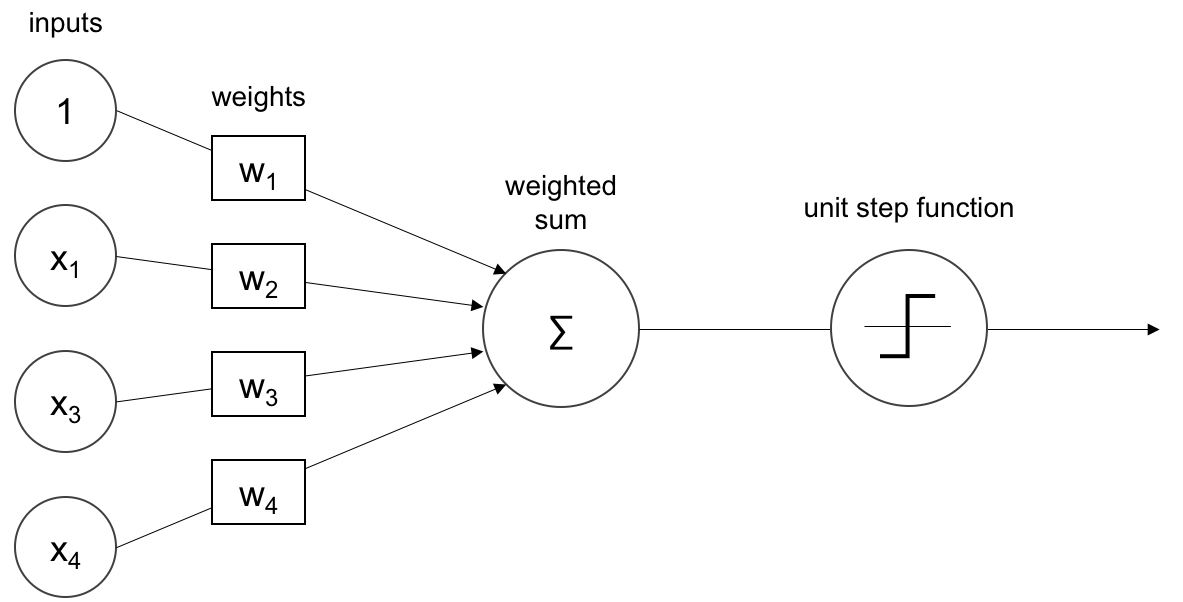
The inputs are weighted and summed as shown in the preceding image. The sum is then passed through a unit step function, in this case, for a binary classification problem. A perceptron can only learn simple functions by learning the weights from examples. The process of learning the weights is called training. The training on a perceptron can be done through gradient-based methods which are explained in a later section. The output of the perceptron can be passed through an activation function or transfer function, which will be explained in the next section.
The activation functions make neural nets nonlinear. An activation function decides whether a perceptron should fire or not. During training activation, functions play an important role in adjusting the gradients. An activation function such as sigmoid, shown in the next section, attenuates the values with higher magnitudes. This nonlinear behaviour of the activation function gives the deep nets to learn complex functions. Most of the activation functions are continuous and differential functions, except rectified unit at 0. A continuous function has small changes in output for every small change in input. A differential function has a derivative existing at every point in the domain.
In order to train a neural network, the function has to be differentiable. Following are a few activation functions.
Note
Don't worry if you don't understand the terms like continuous and differentiable in detail. It will become clearer over the chapters.
Sigmoid can be considered a smoothened step function and hence differentiable. Sigmoid is useful for converting any value to probabilities and can be used for binary classification. The sigmoid maps input to a value in the range of 0 to 1, as shown in the following graph:
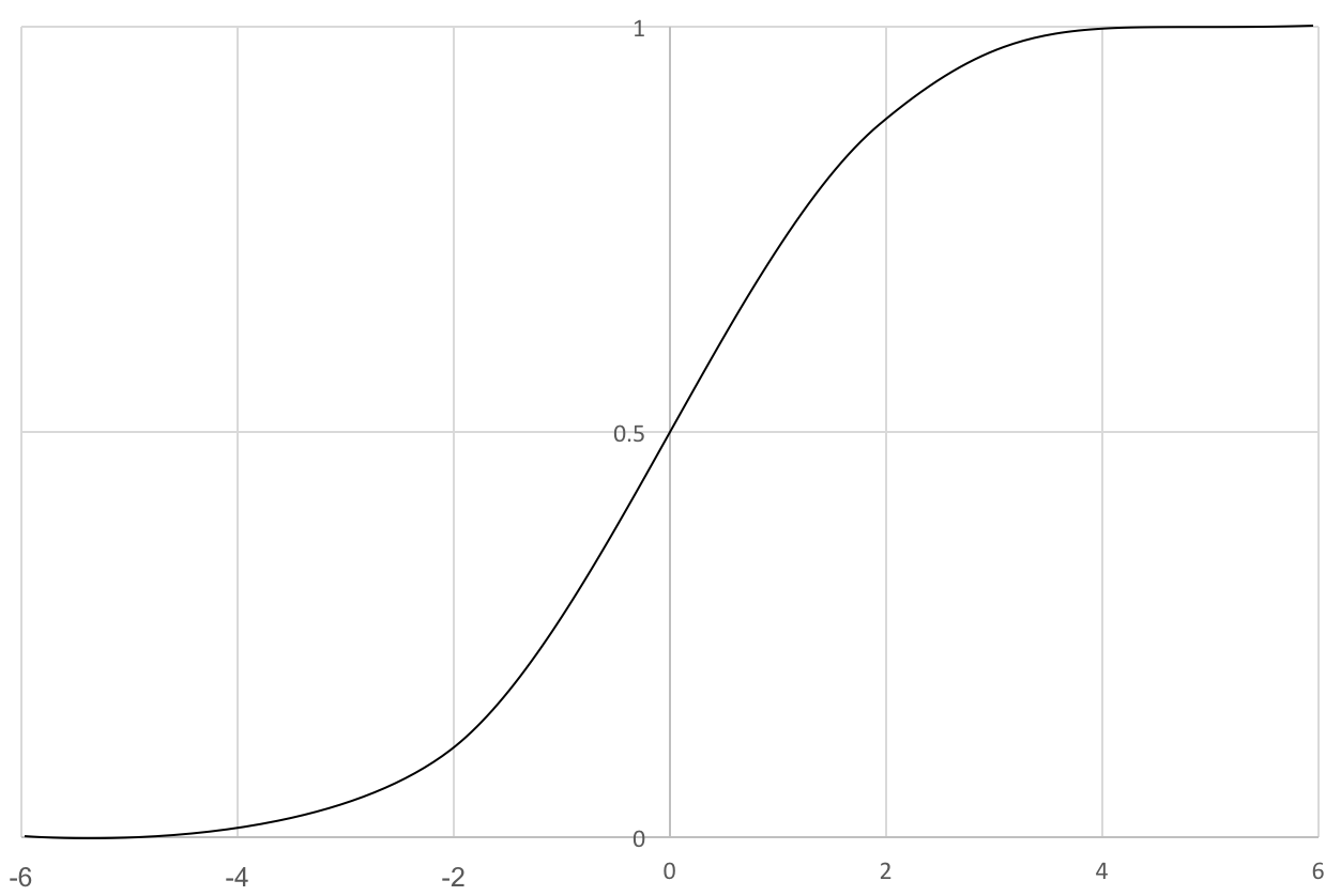
The change in Y values with respect to X is going to be small, and hence, there will be vanishing gradients. After some learning, the change may be small. Another activation function called tanh, explained in next section, is a scaled version of sigmoid and avoids the problem of a vanishing gradient.
The hyperbolic tangent function, or tanh, is the scaled version of sigmoid. Like sigmoid, it is smooth and differentiable. The tanh maps input to a value in the range of -1 to 1, as shown in the following graph:
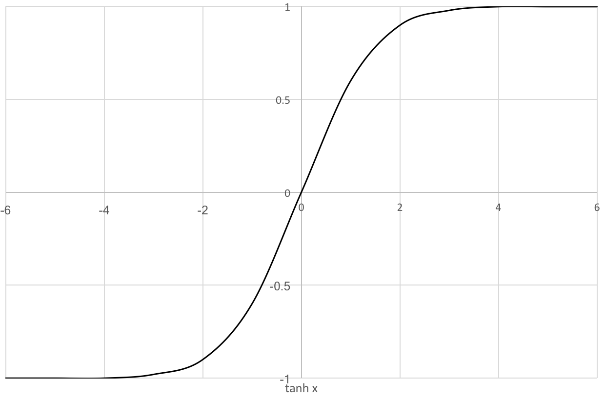
The gradients are more stable than sigmoid and hence have fewer vanishing gradient problems. Both sigmoid and tanh fire all the time, making the ANN really heavy. The Rectified Linear Unit (ReLU) activation function, explained in the next section, avoids this pitfall by not firing at times.
ReLu can let big numbers pass through. This makes a few neurons stale and they don't fire. This increases the sparsity, and hence, it is good. The ReLU maps input x to max (0, x), that is, they map negative inputs to 0, and positive inputs are output without any change as shown in the following graph:
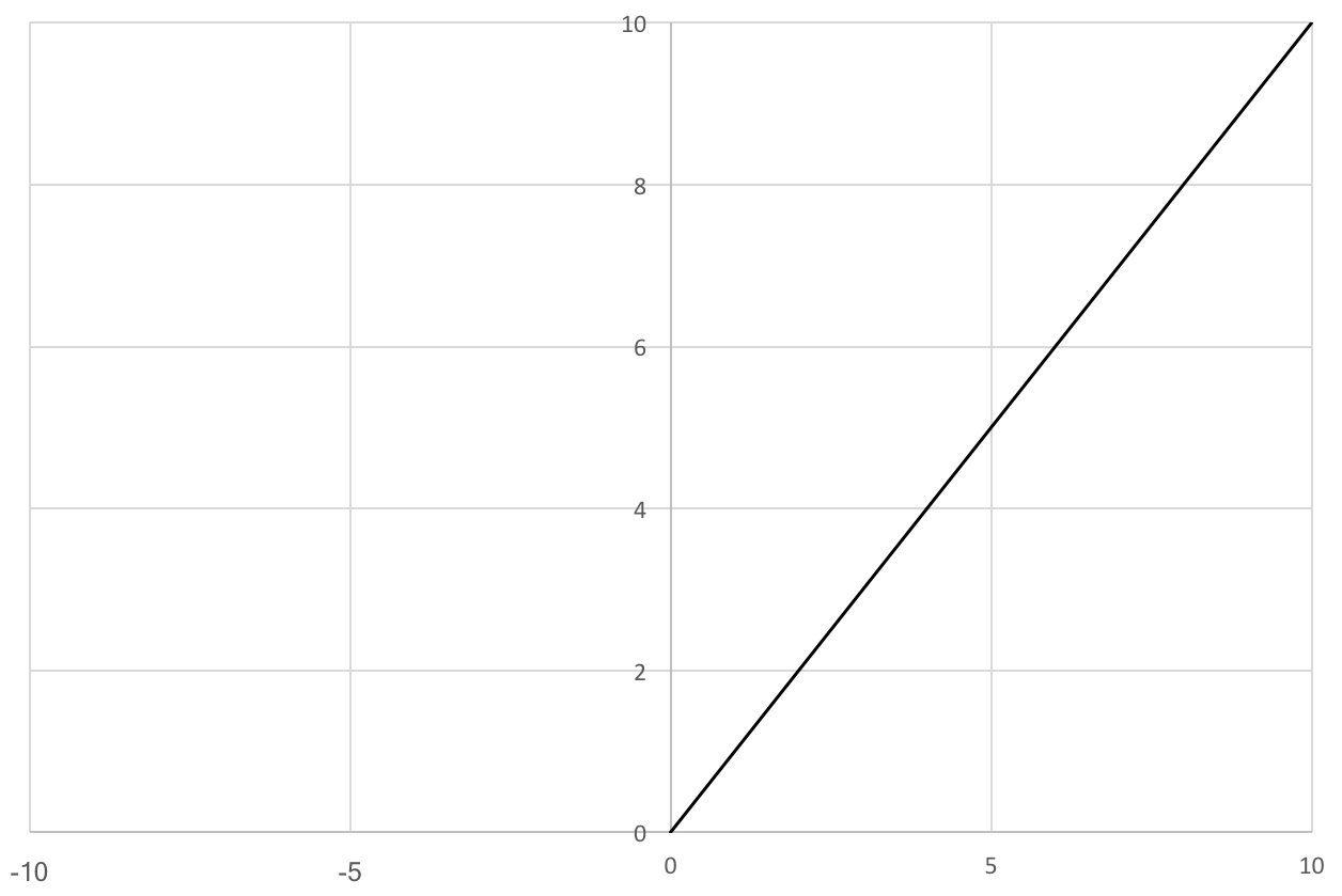
Because ReLU doesn't fire all the time, it can be trained faster. Since the function is simple, it is computationally the least expensive. Choosing the activation function is very dependent on the application. Nevertheless, ReLU works well for a large range of problems. In the next section, you will learn how to stack several perceptrons together that can learn more complex functions than perceptron.
ANN is a collection of perceptrons and activation functions. The perceptrons are connected to form hidden layers or units. The hidden units form the nonlinear basis that maps the input layers to output layers in a lower-dimensional space, which is also called artificial neural networks. ANN is a map from input to output. The map is computed by weighted addition of the inputs with biases. The values of weight and bias values along with the architecture are called model.
The training process determines the values of these weights and biases. The model values are initialized with random values during the beginning of the training. The error is computed using a loss function by contrasting it with the ground truth. Based on the loss computed, the weights are tuned at every step. The training is stopped when the error cannot be further reduced. The training process learns the features during the training. The features are a better representation than the raw images. The following is a diagram of an artificial neural network, or multi-layer perceptron:
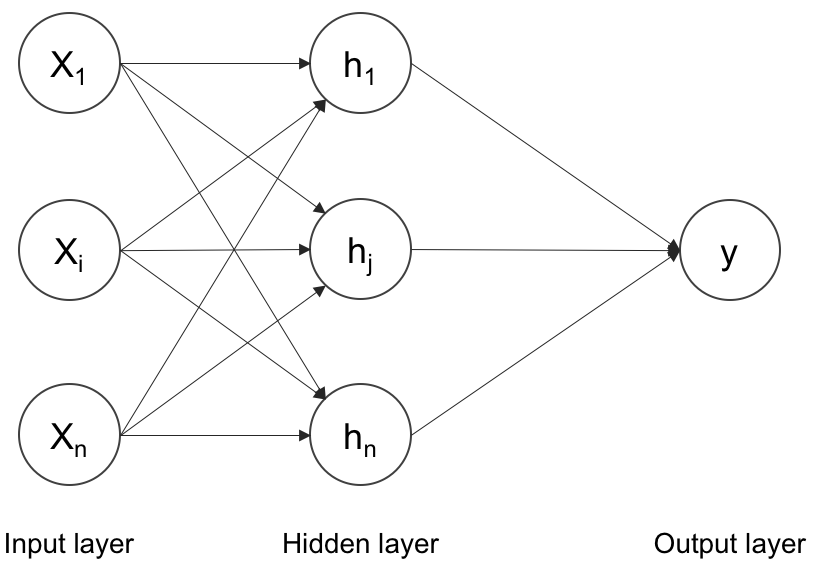
Several inputs of x are passed through a hidden layer of perceptrons and summed to the output. The universal approximation theorem suggests that such a neural network can approximate any function. The hidden layer can also be called a dense layer. Every layer can have one of the activation functions described in the previous section. The number of hidden layers and perceptrons can be chosen based on the problem. There are a few more things that make this multilayer perceptron work for multi-class classification problems. A multi-class classification problem tries to discriminate more than ten categories. We will explore those terms in the following sections.
One-hot encoding is a way to represent the target variables or classes in case of a classification problem. The target variables can be converted from the string labels to one-hot encoded vectors. A one-hot vector is filled with 1 at the index of the target class but with 0 everywhere else. For example, if the target classes are cat and dog, they can be represented by [1, 0] and [0, 1], respectively. For 1,000 classes, one-hot vectors will be of size 1,000 integers with all zeros but 1. It makes no assumptions about the similarity of target variables. With the combination of one-hot encoding with softmax explained in the following section, multi-class classification becomes possible in ANN.
Softmax is a way of forcing the neural networks to output the sum of 1. Thereby, the output values of the softmax function can be considered as part of a probability distribution. This is useful in multi-class classification problems. Softmax is a kind of activation function with the speciality of output summing to 1. It converts the outputs to probabilities by dividing the output by summation of all the other values. The Euclidean distance can be computed between softmax probabilities and one-hot encoding for optimization. But the cross-entropy explained in the next section is a better cost function to optimize.
Cross-entropy compares the distance between the outputs of softmax and one-hot encoding. Cross-entropy is a loss function for which error has to be minimized. Neural networks estimate the probability of the given data to every class. The probability has to be maximized to the correct target label. Cross-entropy is the summation of negative logarithmic probabilities. Logarithmic value is used for numerical stability. Maximizing a function is equivalent to minimizing the negative of the same function. In the next section, we will see the following regularization methods to avoid the overfitting of ANN:
- Dropout
- Batch normalization
- L1 and L2 normalization
Dropout is an effective way of regularizing neural networks to avoid the overfitting of ANN. During training, the dropout layer cripples the neural network by removing hidden units stochastically as shown in the following image:
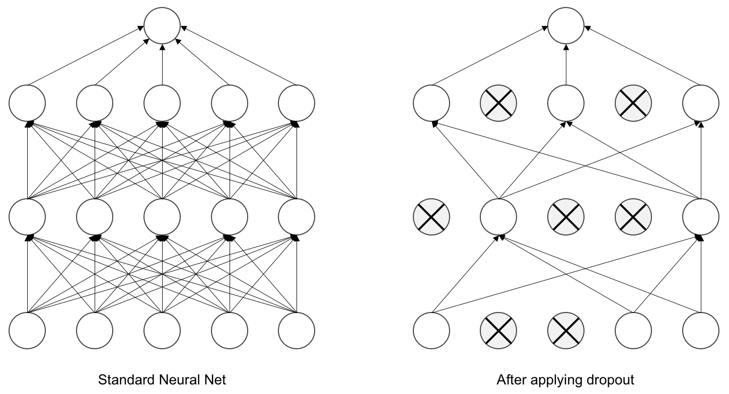
Note how the neurons are randomly trained. Dropout is also an efficient way of combining several neural networks. For each training case, we randomly select a few hidden units so that we end up with different architectures for each case. This is an extreme case of bagging and model averaging. Dropout layer should not be used during the inference as it is not necessary.
Batch normalization, or batch-norm, increase the stability and performance of neural network training. It normalizes the output from a layer with zero mean and a standard deviation of 1. This reduces overfitting and makes the network train faster. It is very useful in training complex neural networks.
Training ANN is tricky as it contains several parameters to optimize. The procedure of updating the weights is called backpropagation. The procedure to minimize the error is called optimization. We will cover both of them in detail in the next sections.
A backpropagation algorithm is commonly used for training artificial neural networks. The weights are updated from backward based on the error calculated as shown in the following image:
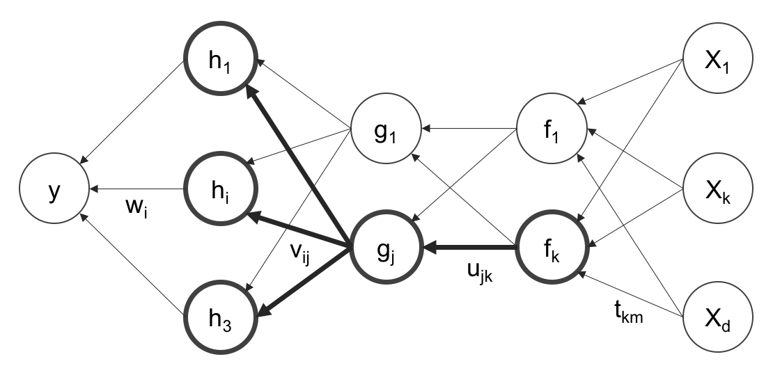
After calculating the error, gradient descent can be used to calculate the weight updating, as explained in the next section.
The gradient descent algorithm performs multidimensional optimization. The objective is to reach the global maximum. Gradient descent is a popular optimization technique used in many machine-learning models. It is used to improve or optimize the model prediction. One implementation of gradient descent is called the stochastic gradient descent (SGD) and is becoming more popular (explained in the next section) in neural networks. Optimization involves calculating the error value and changing the weights to achieve that minimal error. The direction of finding the minimum is the negative of the gradient of the loss function. The gradient descent procedure is qualitatively shown in the following figure:
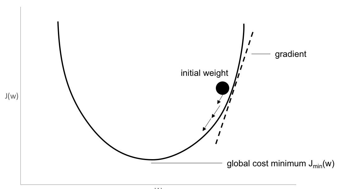
The learning rate determines how big each step should be. Note that the ANN with nonlinear activations will have local minima. SGD works better in practice for optimizing non-convex cost functions.
SGD is the same as gradient descent, except that it is used for only partial data to train every time. The parameter is called mini-batch size. Theoretically, even one example can be used for training. In practice, it is better to experiment with various numbers. In the next section, we will discuss convolutional neural networks that work better on image data than the standard ANN.
Note
Visit https://yihui.name/animation/example/grad-desc/ to see a great visualization of gradient descent on convex and non-convex surfaces.
TensorFlow playground is an interactive visualization of neural networks. Visit http://playground.tensorflow.org/, play by changing the parameters to see how the previously mentioned terms work together. Here is a screenshot of the playground:
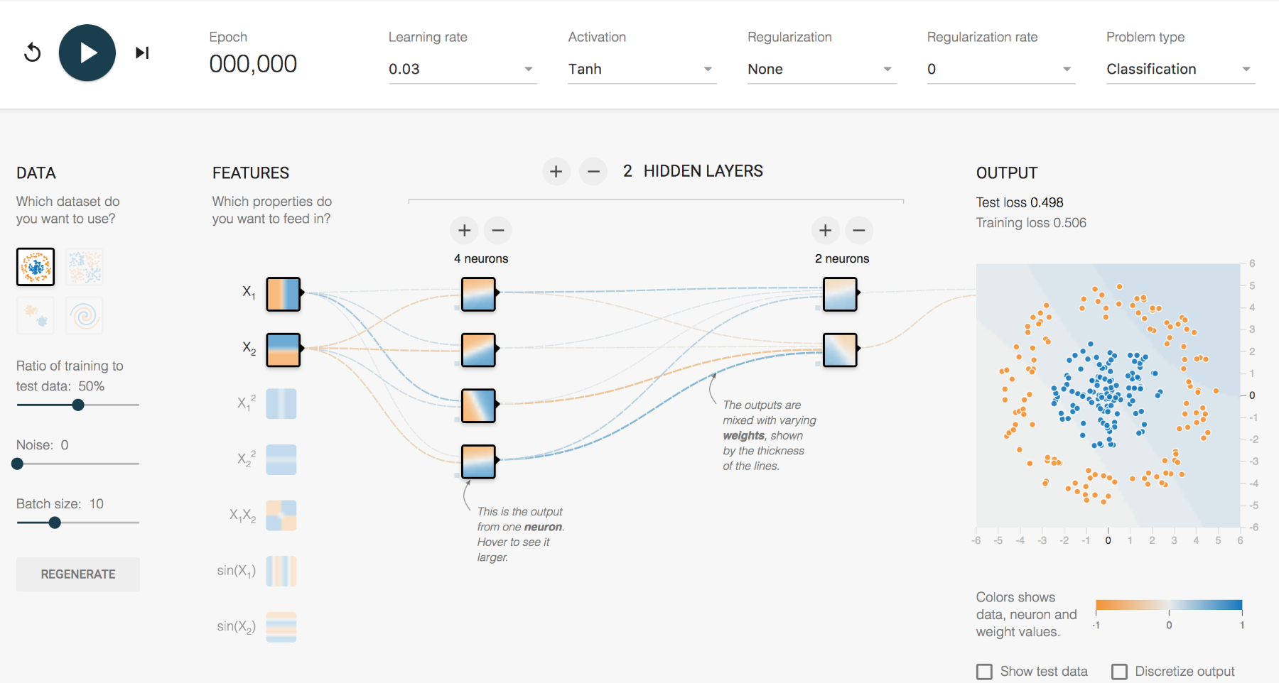
Dashboard in the TensorFlow playground
As shown previously, the reader can change learning rate, activation, regularization, hidden units, and layers to see how it affects the training process. You can spend some time adjusting the parameters to get the intuition of how neural networks for various kinds of data.
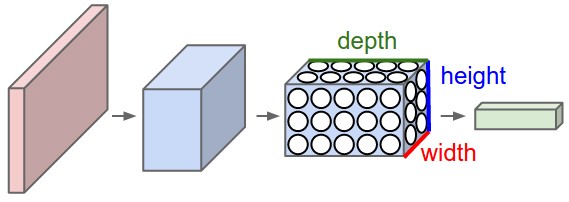
Convolutional neural networks (CNN) are similar to the neural networks described in the previous sections. CNNs have weights, biases, and outputs through a nonlinear activation. Regular neural networks take inputs and the neurons fully connected to the next layers. Neurons within the same layer don't share any connections. If we use regular neural networks for images, they will be very large in size due to a huge number of neurons, resulting in overfitting. We cannot use this for images, as images are large in size. Increase the model size as it requires a huge number of neurons. An image can be considered a volume with dimensions of height, width, and depth. Depth is the channel of an image, which is red, blue, and green. The neurons of a CNN are arranged in a volumetric fashion to take advantage of the volume. Each of the layers transforms the input volume to an output volume as shown in the following image:
Convolution neural network filters encode by transformation. The learned filters detect features or patterns in images. The deeper the layer, the more abstract the pattern is. Some analyses have shown that these layers have the ability to detect edges, corners, and patterns. The learnable parameters in CNN layers are less than the dense layer described in the previous section.
Kernel is the parameter convolution layer used to convolve the image. The convolution operation is shown in the following figure:
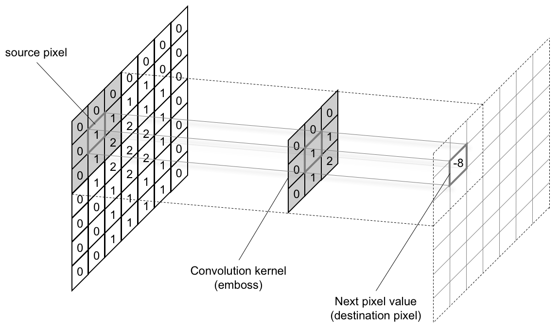
The kernel has two parameters, called stride and size. The size can be any dimension of a rectangle. Stride is the number of pixels moved every time. A stride of length 1 produces an image of almost the same size, and a stride of length 2 produces half the size. Padding the image will help in achieving the same size of the input.
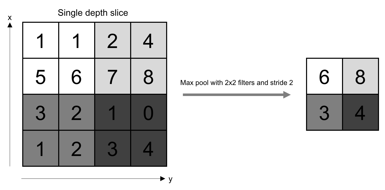
Pooling layers are placed between convolution layers. Pooling layers reduce the size of the image across layers by sampling. The sampling is done by selecting the maximum value in a window. Average pooling averages over the window. Pooling also acts as a regularization technique to avoid overfitting. Pooling is carried out on all the channels of features. Pooling can also be performed with various strides.
The size of the window is a measure of the receptive field of CNN. The following figure shows an example of max pooling:
CNN is the single most important component of any deep learning model for computer vision. It won't be an exaggeration to state that it will be impossible for any computer to have vision without a CNN. In the next sections, we will discuss a couple of advanced layers that can be used for a few applications.
Note
Visit https://www.youtube.com/watch?v=jajksuQW4mc for a great visualization of a CNN and max-pooling operation.
Recurrent neural networks (RNN) can model sequential information. They do not assume that the data points are intensive. They perform the same task from the output of the previous data of a series of sequence data. This can also be thought of as memory. RNN cannot remember from longer sequences or time. It is unfolded during the training process, as shown in the following image:
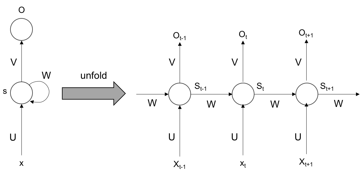
As shown in the preceding figure, the step is unfolded and trained each time. During backpropagation, the gradients can vanish over time. To overcome this problem, Long short-term memory can be used to remember over a longer time period.
Long short-term memory (LSTM) can store information for longer periods of time, and hence, it is efficient in capturing long-term efficiencies. The following figure illustrates how an LSTM cell is designed:
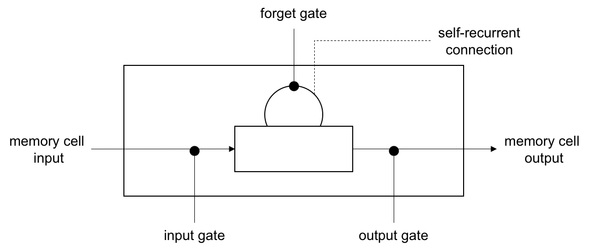
LSTM has several gates: forget, input, and output. Forget gate maintains the information previous state. The input gate updates the current state using the input. The output gate decides the information be passed to the next state. The ability to forget and retain only the important things enables LSTM to remember over a longer time period. You have learned the deep learning vocabulary that will be used throughout the book. In the next section, we will see how deep learning can be used in the context of computer vision.