


The first operation of the model is reading the images and standardizing them. In fact, we cannot work with images of variable sizes; therefore, in this first step, we'll load the images and reshape them to a predefined size (32x32). Moreover, we will one-hot encode the labels in order to have a 43-dimensional array where only one element is enabled (it contains a 1), and we will convert the color space of the images from RGB to grayscale. By looking at the images, it seems obvious that the information we need is not contained in the color of the signal but in its shape and design.
Let's now open a Jupyter Notebook and place some code to do that. First of all, let's create some final variables containing the number of classes (43) and the size of the images after being resized:
N_CLASSES = 43
RESIZED_IMAGE = (32, 32)
Next, we will write a function that reads all the images given in a path, resize them to a predefined shape, convert them to grayscale, and also one-hot encode the label. In order to do that, we'll use a named tuple named dataset:
import matplotlib.pyplot as plt
import glob
from skimage.color import rgb2lab
from skimage.transform import resize
from collections import namedtuple
import numpy as np
np.random.seed(101)
%matplotlib inline
Dataset = namedtuple('Dataset', ['X', 'y'])
def to_tf_format(imgs):
   return np.stack([img[:, :, np.newaxis] for img in imgs], axis=0).astype(np.float32)
def read_dataset_ppm(rootpath, n_labels, resize_to):
images = []
labels = []
for c in range(n_labels):
   full_path = rootpath + '/' + format(c, '05d') + '/'
   for img_name in glob.glob(full_path + "*.ppm"):

     img = plt.imread(img_name).astype(np.float32)
     img = rgb2lab(img / 255.0)[:,:,0]
     if resize_to:
       img = resize(img, resize_to, mode='reflect')

     label = np.zeros((n_labels, ), dtype=np.float32)
     label[c] = 1.0
    images.append(img.astype(np.float32))
     labels.append(label)
return Dataset(X = to_tf_format(images).astype(np.float32),
                 y = np.matrix(labels).astype(np.float32))
dataset = read_dataset_ppm('GTSRB/Final_Training/Images', N_CLASSES, RESIZED_IMAGE)
print(dataset.X.shape)
print(dataset.y.shape)
Thanks to the skimage module, the operation of reading, transforming, and resizing is pretty easy. In our implementation, we decided to convert the original color space (RGB) to lab, then retaining only the luminance component. Note that another good conversion here is YUV, where only the "Y" component should be retained as a grayscale image.
Running the preceding cell gives this:
(39209, 32, 32, 1)
(39209, 43)
One note about the output format: the shape of the observation matrix X has four dimensions. The first indexes the observations (in this case, we have almost 40,000 of them); the other three dimensions contain the image (which is 32 pixel, by 32 pixels grayscale, that is, one-dimensional). This is the default shape when dealing with images in TensorFlow (see the code _tf_format function).
As for the label matrix, the rows index the observation, while the columns are the one-hot encoding of the label.
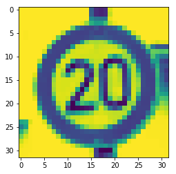
In order to have a better understanding of the observation matrix, let's print the feature vector of the first sample, together with its label:
plt.imshow(dataset.X[0, :, :, :].reshape(RESIZED_IMAGE)) #sample
print(dataset.y[0, :]) #label
[[1. 0. 0. 0. 0. 0. 0. 0. 0. 0. 0. 0. 0. 0. 0. 0. 0. 0. 0. 0. 0. 0. 0. 0.
0. 0. 0. 0. 0. 0. 0. 0. 0. 0. 0. 0. 0. 0. 0. 0. 0. 0.]]
You can see that the image, that is, the feature vector, is 32x32. The label contains only one 1 in the first position.
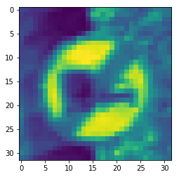
Let's now print the last sample:
plt.imshow(dataset.X[-1, :, :, :].reshape(RESIZED_IMAGE)) #sample
print(dataset.y[-1, :]) #label
[[0. 0. 0. 0. 0. 0. 0. 0. 0. 0. 0. 0. 0. 0. 0. 0. 0. 0. 0. 0. 0. 0. 0. 0.
0. 0. 0. 0. 0. 0. 0. 0. 0. 0. 0. 0. 0. 0. 0. 0. 0. 1.]]
The feature vector size is the same (32x32), and the label vector contains one 1 in the last position.
These are the two pieces of information we need to create the model. Please, pay particular attention to the shapes, because they're crucial in deep learning while working with images; in contrast to classical machine learning observation matrices, here the X has four dimensions!
The last step of our preprocessing is the train/test split. We want to train our model on a subset of the dataset, and then measure the performance on the leftover samples, that is, the test set. To do so, let's use the function provided by sklearn:
from sklearn.model_selection import train_test_split
idx_train, idx_test = train_test_split(range(dataset.X.shape[0]), test_size=0.25, random_state=101)
X_train = dataset.X[idx_train, :, :, :]
X_test = dataset.X[idx_test, :, :, :]
y_train = dataset.y[idx_train, :]
y_test = dataset.y[idx_test, :]
print(X_train.shape)
print(y_train.shape)
print(X_test.shape)
print(y_test.shape)
In this example, we'll use 75% of the samples in the dataset for training and the remaining 25% for testing. In fact, here's the output of the previous code:
(29406, 32, 32, 1)
(29406, 43)
(9803, 32, 32, 1)
(9803, 43)


