


Convolutional neural networks (CNNs) utilize convolutional operations to extract useful information from data that has a topology associated with it. This works best for image and audio data. The input image, when passed through a convolution layer, produces several output images, known as output feature maps. The output feature maps detect features. The output feature maps in the initial convolutional layer may learn to detect basic features, such as edges and color composition variation.
The second convolutional layer may detect slightly more complicated features, such as squares, circles, and other geometrical structures. As we progress through the neural network, the convolutional layers learn to detect more and more complicated features. For instance, if we have a CNN that classifies whether an image is of a cat or a dog, the convolutional layers at the bottom of the neural network might learn to detect features such as the head, the legs, and so on.
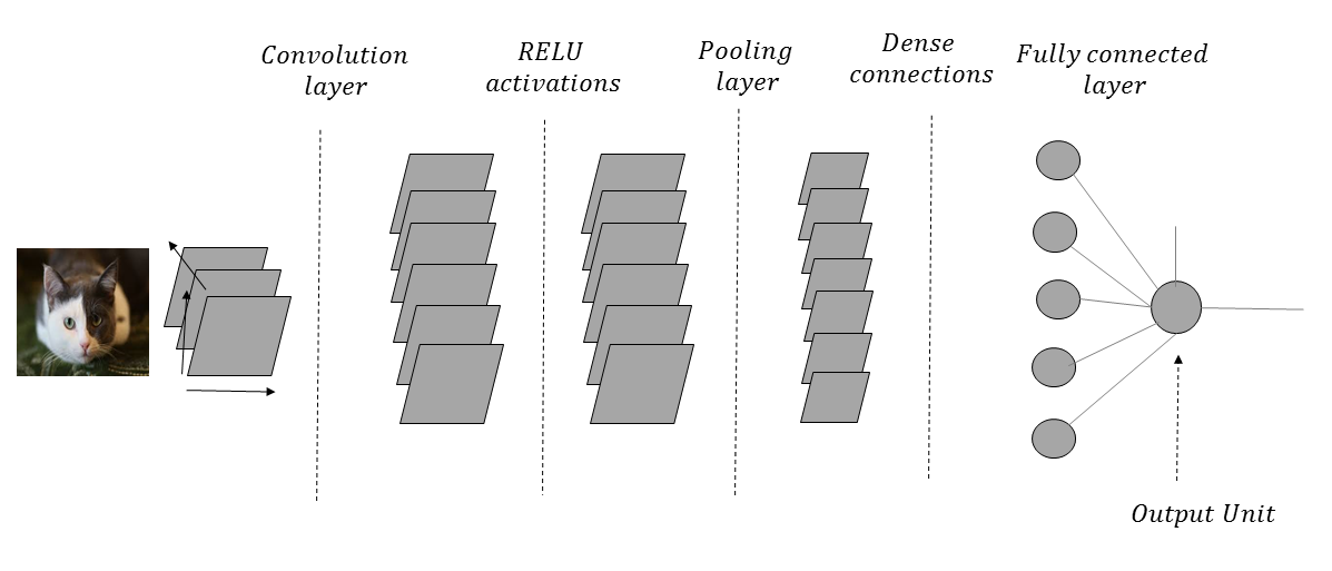
Figure 1.11 shows an architectural diagram of a CNN that processes images of cats and dogs in order to classify them. The images are passed through a convolutional layer that helps to detect relevant features, such as edges and color composition. The ReLU activations add nonlinearity. The pooling layer that follows the activation layer summarizes local neighborhood information in order to provide an amount of translational invariance. In an ideal CNN, this convolution-activation-pooling operation is performed several times before the network makes its way to the dense connections:
As we go through such a network with several convolution-activation-pooling operations, the spatial resolution of the image is reduced, while the number of output feature maps is increased in every layer. Each output feature map in a convolutional layer is associated with a filter kernel, the weights of which are learned through the CNN training process.
In a convolutional operation, a flipped version of a filter kernel is laid over the entire image or feature map, and the dot product of the filter-kernel input values with the corresponding image pixel or the feature map values are computed for each location on the input image or feature map. Readers that are already accustomed to ordinary image processing may have used different filter kernels, such as a Gaussian filter, a Sobel edge detection filter, and many more, where the weights of the filters are predefined. The advantage of convolutional neural networks is that the different filter weights are determined through the training process; This means that, the filters are better customized for the problem that the convolutional neural network is dealing with.
When a convolutional operation involves overlaying the filter kernel on every location of the input, the convolution is said to have a stride of one. If we choose to skip one location while overlaying the filter kernel, then convolution is performed with a stride of two. In general, if n locations are skipped while overlaying the filter kernel over the input, the convolution is said to have been performed with a stride of (n+1). Strides of greater than one reduce the spatial dimensions of the output of the convolution.
Generally, a convolutional layer is followed by a pooling layer, which basically summarizes the output feature map activations in a neighborhood, determined by the receptive field of the pooling. For instance, a 2 x 2 receptive field will gather the local information of four neighboring output feature map activations. For max-pooling operations, the maximum value of the four activations is selected as the output, while for average pooling, the average of the four activations is selected. Pooling reduces the spatial resolution of the feature maps. For instance, for a 224 x 224 sized feature map pooling operation with a 2 x 2 receptive field, the spatial dimension of the feature map will be reduced to 112 x 112.
One thing to note is that a convolutional operation reduces the number of weights to be learned in each layer. For instance, if we have an input image of a spatial dimension of 224 x 224 and the desired output of the next layer is of the dimensions 224 x 224, then for a traditional neural network with full connections, the number of weights to be learned is 224 x 224 x 224 x 224. For a convolutional layer with the same input and output dimensions, all that we need to learn are the weights of the filter kernel. So, if we use a 3 x 3 filter kernel, we just need to learn nine weights as opposed to 224 x 224 x 224 x 224 weights. This simplification works, since structures like images and audio in a local spatial neighborhood have high correlation among them.
The input images pass through several layers of convolutional and pooling operations. As the network progresses, the number of feature maps increases, while the spatial resolution of the images decreases. At the end of the convolutional-pooling layers, the output of the feature maps is fed to the fully connected layers, followed by the output layer.
The output units are dependent on the task at hand. If we are performing regression, the output activation unit is linear, while if it is a binary classification problem, the output unit is a sigmoid. For multi-class classification, the output layer is a softmax unit.
In all of the image processing projects in this book, we will use convolutional neural networks, in one form or another.


