In this section, I will introduce the main libraries in Python's data science stack. These will be our computational tools. Although proficiency in them is not a prerequisite for following the contents of this book, knowledge of them will certainly be useful. My goal is not to provide complete coverage of these tools, as there are many excellent resources and tutorials for that purpose; here, I just want to introduce some of the basic concepts about them and in the following chapters of the book we will see how to use these tools for doing predictive analytics. If you are already familiar with these tools you can, of course, skip this section.

Here's the description of Anaconda from the official site:

The analogy that I like to make is that Anaconda is like a toolbox: a ready-to-use collection of related tools for doing analytics and scientific computing with Python. You can certainly go ahead and get the individual tools one by one, but it is definitely more convenient to get the whole toolbox rather than getting them individually. Anaconda also takes care of package dependencies and other potential conflicts and pains of installing Python packages individually. Installing the main libraries (and dependencies) for predictive analytics will probably end up causing conflicts that are painful to deal with. It's difficult to keep packages from interacting with each other, and more difficult to keep them all updated. Anaconda makes getting and maintaining all these packages quick and easy.

It is not required, but I strongly recommend using Anaconda with this book, otherwise you will need to install all the libraries we will be using individually. The installation process of Anaconda is as easy as installing any other software on your computer, so if you don’t have it already please go to https://www.anaconda.com/download/ and look for the downloader for your operating system. Please use Python version 3.6, which is the latest version at the time of writing. Although many companies and systems are still using Python 2.7, the community has been making a great effort to transition to Python 3, so let's move forward with them.

One last thing about Anaconda—if you want to learn more about it, please refer to the documentation at https://docs.anaconda.com/anaconda/.

Since we will be working with code, we will need a tool to write it. In principle, you can use one of the many IDEs available for Python, however, Jupyter Notebooks have become the standard for analytics and data science professionals:

Jupyter comes with Anaconda; it is really easy to use. Following are the steps:

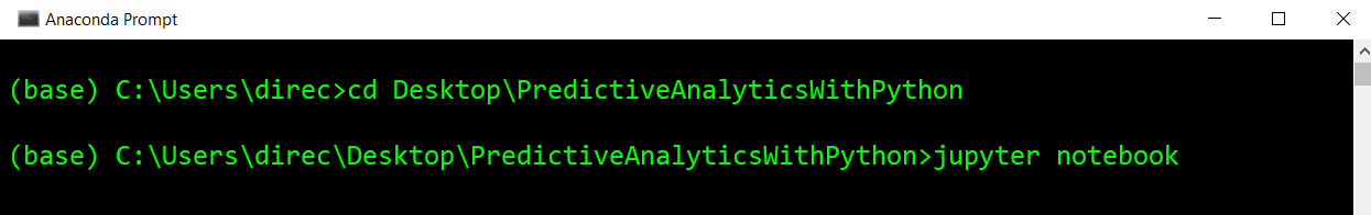
1. Just open the Anaconda prompt, navigate to the directory where you want to start the application (in my case it is in Desktop | PredictiveAnalyticsWithPython), and type jupyter notebook to start the application:

You will see something that looks like this:

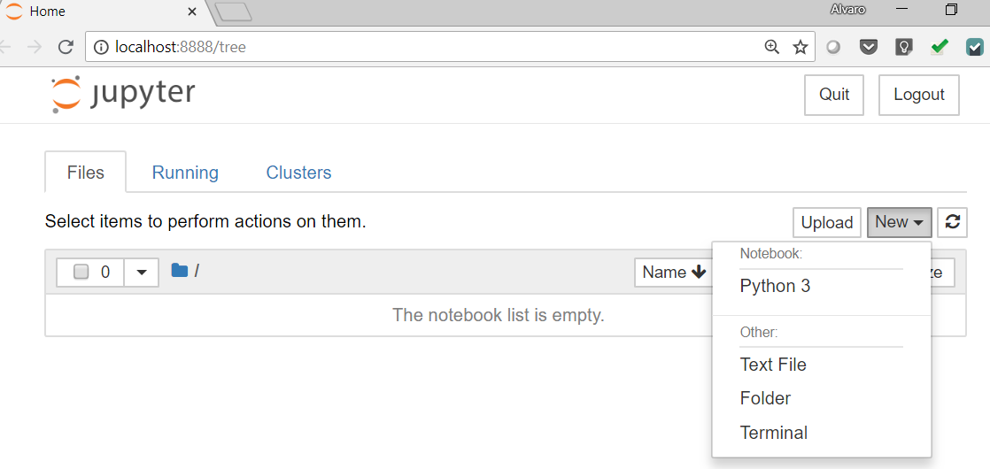
2. Go to New | Python 3. A new browser window will open. Jupyter Notebook is a web application that consists of cells. There are two types of cells: Markdown and Code cells. In Markdown, you can write formatted text and insert images, links, and other elements. Code cells are the default type.
3. To change to markdown in the main menu, go to Cell | Cell Type | Markdown. When you are editing markdown cells, they look like this:

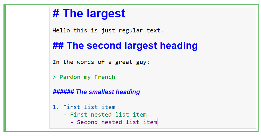
And the result would look like this:

You can find a complete guide to markdown syntax here: https://help.github.com/articles/basic-writing-and-formatting-syntax/.

4. On the other hand, in code cells you can write and execute Python code, and the result of the execution will be displayed; to execute the code, the keyboard shortcut is Ctrl + Enter:

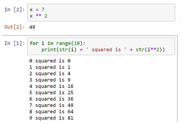
We will use Jupyter Notebooks in most of the examples of the book (sometimes we will use the regular Python shell for simplicity).

5. In the main Notebook menu, go to Help and there you can find a User Interface Tour, Keyboard Shortcuts, and other interesting resources. Please take a look at them if you are just getting familiar with Jupyter.

Finally, at the time of writing, the Jupyter Lab is the next project of the Jupyter community. It offers additional functionality; you can also try it if you want—the notebooks of this book will run there too.

NumPy is the foundational library for the scientific computing library for the Python ecosystem; the main libraries in the ecosystem—pandas, matplotlib, SciPy, and scikit-learn—are based on NumPy.

As it is a foundational library, it is important to know at least the basics of NumPy. Let's have a mini tutorial on NumPy.

Here are a couple of little motivating examples about why we need vectorization when doing any kind of scientific computing. You will see what we mean by vectorization in the following example.

Let's perform a couple of simple calculations with Python. We have two examples:

• First, let's say we have some distances and times and we would like to calculate the speeds:

distances = [10, 15, 17, 26]
times = [0.3, 0.47, 0.55, 1.20]
# Calculate speeds with Python
speeds = []
for i in range(4):
    speeds.append(distances[i]/times[i])

speeds

Here we have the speeds:

[33.333333333333336,
 31.914893617021278,
 30.909090909090907,
 21.666666666666668]

An alternative to accomplish the same in Python methodology would be the following:

# An alternative
speeds = [d/t for d,t in zip(distances, times)]

• For our second motivating example, let's say we have a list of product quantities and their respective prices and that we would like to calculate the total of the purchase. The code in Python would look something like this:

product_quantities = [13, 5, 6, 10, 11]
prices = [1.2, 6.5, 1.0, 4.8, 5.0]
total = sum([q*p for q,p in zip(product_quantities, prices)])
total

This will give a total of 157.1.

The point of these examples is that, for this type of calculation, we need to perform operations element by element and in Python (and most programming languages) we do it by using for loops or list comprehensions (which are just convenient ways of writing for loops). Vectorization is a style of computer programming where operations are applied to arrays of individual elements; in other words, a vectorized operation is the application of the operation, element by element, without explicitly doing it with for loops.

Now let's take a look at the NumPy approach to doing the former operations:

1. First, let's import the library:

import numpy as np

2. Now let's do the speeds calculation. As you can see, this is very easy and natural: just add the mathematical definition of speed:

# calculating speeds
distances = np.array([10, 15, 17, 26])
times = np.array([0.3, 0.47, 0.55, 1.20])
speeds = distances / times
speeds

This is what the output looks like:

array([ 33.33333333,  31.91489362,  30.90909091,  21.66666667])

Now, the purchase calculation. Again, the code for running this calculation is much easier and more natural:

#Calculating the total of a purchase
product_quantities = np.array([13, 5, 6, 10, 11])
prices = np.array([1.2, 6.5, 1.0, 4.8, 5.0])
total = (product_quantities*prices).sum()
total

After running this calculation, you will see that we get the same total: 157.1.

Now let's talk about some of the basics of array creation, main attributes, and operations. This is of course by no means a complete introduction, but it will be enough for you to have a basic understanding of how NumPy arrays work.

As we saw before, we can create arrays from lists like so:

# arrays from lists
distances = [10, 15, 17, 26, 20]
times = [0.3, 0.47, 0.55, 1.20, 1.0]
distances = np.array(distances)
times = np.array(times)

If we pass a list of lists to np.array(), it will create a two-dimensional array. If passed a list of lists of lists (three nested lists), it will create a three-dimensional array, and so on and so forth:

A = np.array([[1, 2], [3, 4]])

This is how A looks:

array([[1, 2], [3, 4]])

Take a look at some of the array's main attributes. Let's create some arrays containing randomly generated numbers:

np.random.seed(0) # seed for reproducibility
x1 = np.random.randint(low=0, high=9, size=12) # 1D array
x2 = np.random.randint(low=0, high=9, size=(3, 4)) # 2D array
x3 = np.random.randint(low=0, high=9, size=(3, 4, 5)) # 3D array
print(x1, '\n')
print(x2, '\n')
print(x3, '\n')

Here are our arrays:

[5 0 3 3 7 3 5 2 4 7 6 8] 

[[8 1 6 7]
 [7 8 1 5]
 [8 4 3 0]] 

[[[3 5 0 2 3]
  [8 1 3 3 3]
  [7 0 1 0 4]
  [7 3 2 7 2]]

 [[0 0 4 5 5]
  [6 8 4 1 4]
  [8 1 1 7 3]
  [6 7 2 0 3]]

 [[5 4 4 6 4]
  [4 3 4 4 8]
  [4 3 7 5 5]
  [0 1 5 3 0]]] 

Important array attributes are the following:

• ndarray.ndim: The number of axes (dimensions) of the array.
• ndarray.shape: The dimensions of the array. This tuple of integers indicates the size of the array in each dimension.
• ndarray.size: The total number of elements of the array. This is equal to the product of the elements of shape.
• ndarray.dtype: An object describing the type of the elements in the array. One can create or specify dtype's using standard Python types. Also, NumPy provides types of its own. numpy.int32, numpy.int16, and numpy.float64 are some examples:

print("x3 ndim: ", x3.ndim)
print("x3 shape:", x3.shape)
print("x3 size: ", x3.size)
print("x3 size: ", x3.dtype)

The output is as follows:

x3 ndim:  3
x3 shape: (3, 4, 5)
x3 size:  60
x3 size:  int32

One-dimensional arrays can be indexed, sliced, and iterated over, just like lists or other Python sequences:

>>> x1
array([5, 0, 3, 3, 7, 3, 5, 2, 4, 7, 6, 8])
>>> x1[5] # element with index 5
3
>>> x1[2:5] # slice from of elements in indexes 2,3 and 4
array([3, 3, 7])
>>> x1[-1] # the last element of the array
8

Multi-dimensional arrays have one index per axis. These indices are given in a tuple separated by commas:

one_to_twenty = np.arange(1,21) # integers from 1 to 20
>>> my_matrix = one_to_twenty.reshape(5,4) # transform to a 5-row by 4-
column matrix
>>> my_matrix
array([[ 1, 2, 3, 4],
[ 5, 6, 7, 8],
[ 9, 10, 11, 12],
[13, 14, 15, 16],
[17, 18, 19, 20]])
>>> my_matrix[2,3] # element in row 3, column 4 (remember Python is zeroindexed)
12
>>> my_matrix[:, 1] # each row in the second column of my_matrix
array([ 2, 6, 10, 14, 18])
>>> my_matrix[0:2,-1] # first and second row of the last column
array([4, 8])
>>> my_matrix[0,0] = -1 # setting the first element to -1
>>> my_matrix

The output of the preceding code is as follows:

array([[-1, 2, 3, 4],
 [ 5, 6, 7, 8],
 [ 9, 10, 11, 12],
 [13, 14, 15, 16],
 [17, 18, 19, 20]])

Finally, let's perform some mathematical operations on the former matrix, just to have some examples of how vectorization works:

>>> one_to_twenty = np.arange(1,21) # integers from 1 to 20
>>> my_matrix = one_to_twenty.reshape(5,4) # transform to a 5-row by 4-
column matrix
>>> # the following operations are done to every element of the matrix
>>> my_matrix + 5 # addition
array([[ 6, 7, 8, 9],
 [10, 11, 12, 13],
 [14, 15, 16, 17],
 [18, 19, 20, 21],
 [22, 23, 24, 25]])
>>> my_matrix / 2 # division
array([[ 0.5, 1. , 1.5, 2. ],
 [ 2.5, 3. , 3.5, 4. ],
 [ 4.5, 5. , 5.5, 6. ],
 [ 6.5, 7. , 7.5, 8. ],
 [ 8.5, 9. , 9.5, 10. ]])
>>> my_matrix ** 2 # exponentiation
array([[ 1, 4, 9, 16],
 [ 25, 36, 49, 64],
 [ 81, 100, 121, 144],
 [169, 196, 225, 256],
 [289, 324, 361, 400]], dtype=int32)
>>> 2**my_matrix # powers of 2
array([[ 2, 4, 8, 16],
 [ 32, 64, 128, 256],
 [ 512, 1024, 2048, 4096],
 [ 8192, 16384, 32768, 65536],
 [ 131072, 262144, 524288, 1048576]], dtype=int32)
>>> np.sin(my_matrix) # mathematical functions like sin
array([[ 0.84147098, 0.90929743, 0.14112001, -0.7568025 ],
       [-0.95892427, -0.2794155 , 0.6569866 , 0.98935825],
       [ 0.41211849, -0.54402111, -0.99999021, -0.53657292],
       [ 0.42016704, 0.99060736, 0.65028784, -0.28790332],
       [-0.96139749, -0.75098725, 0.14987721, 0.91294525]])

Finally, let's take a look at some useful methods commonly used in data analysis:

>>> # some useful methods for analytics
>>> my_matrix.sum()
210
>>> my_matrix.max() ## maximum
20
>>> my_matrix.min() ## minimum
1
>>> my_matrix.mean() ## arithmetic mean
10.5
>>> my_matrix.std() ## standard deviation
5.766281297335398

I don't want to reinvent the wheel here; there are many excellent resources on the basics of NumPy.

SciPy is a collection of sub-packages for many specialized scientific computing tasks.

The sub-packages available in SciPy are summarized in the following table:

We will introduce some functions and sub-packages of SciPy as we need them in the next chapters.

Pandas was fundamentally created for working with two types of data structures. For one-dimensional data, we have the Series. The most common use of Pandas is the two-dimensional structure, called the DataFrame; think of it as an SQL table or as an Excel spreadsheet.

Although there are other data structures, with these two we can cover more than 90% of the use cases in predictive analytics. In fact, most of the time (and in all the examples of the book) we will work with DataFrames. We will introduce the basic functionality of pandas in the next chapter, not explicitly, but by doing.

This is the main library for producing 2D visualizations and is one of the oldest scientific computing tools in the Python ecosystem. Although there is an increasing number of libraries for visualization for Python, Matplotlib is still widely used and actually incorporated into the pandas functionality; in addition, other more specialized visualization projects such as Seaborn are based on Matplotlib.

In this book, we will use base matplotlib only when needed, because we will prefer to use higher-level libraries, especially Seaborn and pandas (which includes great functions for plotting). However, since both of these libraries are built on top of matplotlib, we need to be familiar with some of the basic terminology and concepts of matplotlib because frequently we will need to make modifications to the objects and plots produced by those higher-level libraries. Now let's introduce some of the basics we need to know about this library so we can get started visualizing data. Let's import the library as is customary when working in analytics:

import matplotlib.pyplot as plt
%matplotlib inline # This is necessary for showing the figures in the notebook

First, we have two important objects—figures subplots (also known as axes). The diagram is the top-level container for all plot elements and is the container of subplots. One diagram can have many subplots and each subplot belongs to a single diagram. The following code produces a diagram (which is not seen) with a single empty subplot. Each subplot has many elements such as a y-axis, x-axis, and a title:

fig, ax = plt.subplots()
ax.plot();

This looks like the following:

A diagram with four subplots would be produced by the following code:

fig, axes = plt.subplots(ncols=2, nrows=2)
fig.show();

The output is shown in the following screenshot:

One important thing to know about matplotlib is that it can be confusing for the beginner because there are two ways (interfaces) of using it—Pyplot and the Object Oriented Interface (OOI). I prefer to use the OOI because it makes explicit the object you are working with. The formerly produced axes object is a NumPy array containing the four subplots. Let's plot some random numbers just to show you how we can refer to each of the subplots. The following plots may look different when you run the code. Since we produced random numbers, we can control that by setting a random seed, which we will do later in the book:

fig, axes = plt.subplots(ncols=2, nrows=2)
axes[0,0].set_title('upper left')
axes[0,0].plot(np.arange(10), np.random.randint(0,10,10))

axes[0,1].set_title('upper right')
axes[0,1].plot(np.arange(10), np.random.randint(0,10,10))

axes[1,0].set_title('lower left')
axes[1,0].plot(np.arange(10), np.random.randint(0,10,10))

axes[1,1].set_title('lower right')
axes[1,1].plot(np.arange(10), np.random.randint(0,10,10))
fig.tight_layout(); ## this is for getting nice spacing between the subplots

The output is as follows:

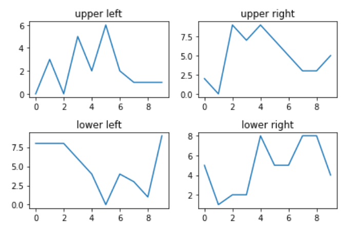
Since the axes object is a NumPy array, we refer to each of the subplots using the NumPy indexation, then we use methods such as .set_title() or .plot() on each subplot to modify it as we would like. There are many of those methods and most of them are used to modify elements of a subplot. For example, the following is almost the same code as before, but written in a way that is a bit more compact and we have modified the y-axis's tick marks.

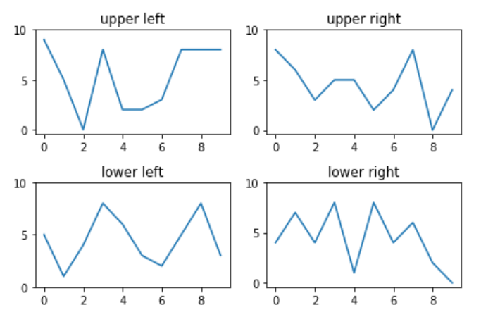
The other API, pyplot, is the one you will find in most of the online examples, .including in the documentation. This is the code to reproduce the above plots using pyplot:

titles = ['upper left', 'upper right', 'lower left', 'lower right']
fig, axes = plt.subplots(ncols=2, nrows=2)
for title, ax in zip(titles, axes.flatten()):
    ax.set_title(title)
    ax.plot(np.arange(10), np.random.randint(0,10,10))
    ax.set_yticks([0,5,10])
    
fig.tight_layout();

The output is as follows:

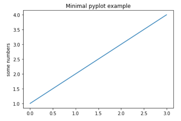
The following code is a minimal example of pyplot:

plt.plot([1,2,3,4])
plt.title('Minimal pyplot example')
plt.ylabel('some numbers')

The following screenshot shows the output:

We won't use pyplot (except for a couple of times) in the book and it will be clear from the context what we do with those functions.

This is a high-level visualization library that specializes in producing statistical plots commonly used in data analysis. The advantage of using Seaborn is that with very few lines of code it can produce highly complex multi-variable visualizations, which are, by the way, very pretty and professional-looking.

The Seaborn library helps us in creating attractive and informative statistical graphics in Python. It is built on top of matplotlib, with a tight PyData stack integration. It supports NumPy and pandas data structures and statistical routines from SciPy and statsmodels.

Seaborn aims to make visualization a central part of exploring and understanding data. The plotting functions operate on DataFrames and arrays containing a complete dataset, which is why it is easier to work with Seaborn when doing data analysis.

We will use Seaborn through the book; we will introduce a lot of useful visualizations, especially in Chapter 3, Dataset Understanding – Exploratory Data Analysis.

This is the main library for traditional machine learning in the Python ecosystem. It offers a consistent and simple API not only to build Machine Learning models but for doing many related tasks such as data pre-processing, transformations, and hyperparameter tuning. It is built on top of NumPy, SciPy, and matplotlib (another reason to know the basics of these libraries) and it is one of the community's favorite tools for doing predictive analytics. We will learn more about this library in Chapter 5, Predicting Categories with Machine Learning, and Chapter 6, Introducing Neural Nets for Predictive Analytics.

TensorFlow is Google's specialized library for deep learning. Open sourced in November 2015, it has become the main library for Deep Learning for both research and production applications in many industries.

TensorFlow includes many advanced computing capabilities and is based on a dataflow programming paradigm. TensorFlow programs work by first building a computational graph and then running the computations described in the graph within specialized objects called "sessions", which are in charge of placing the computations onto devices such as CPUs or GPUs. This computing paradigm is not as straightforward to use and understand (especially for beginners), which is why we won't use TensorFlow directly in our examples. We will use TensorFlow as a "backend" for our computations in Chapter 6, Introducing Neural Nets for Predictive Analytics.

Instead of using TensorFlow directly, we will use Keras to build Deep Learning models. Keras is a great, user-friendly library that serves as a "frontend" for TensorFlow (or other Deep Learning libraries such as Theano). The main goal of Keras is to be "Deep Learning for humans"; in my opinion, Keras fulfills this goal because it makes the development of deep learning models easy and intuitive.

Keras will be our tool of choice in Chapter 6, Introducing Neural Nets for Predictive Analytics, where we will learn about its basic functionality.

Dash is a Python framework for building web applications quickly and easily without knowing Javascript, CSS, HTML, server-side programming, or related technologies that belong to the web development world.