Tensors are the workhorse of PyTorch. If you know linear algebra, they are equivalent to a matrix. Torch tensors are effectively an extension of the numpy.array object. Tensors are an essential conceptual component in deep learning systems, so having a good understanding of how they work is important.

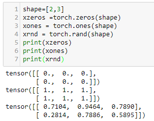
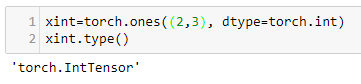
In our first example, we will be looking at tensors of size 2 x 3. In PyTorch, we can create tensors in the same way that we create NumPy arrays. For example, we can pass them nested lists, as shown in the following code:

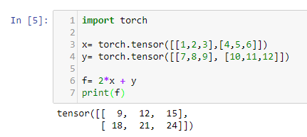
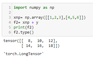
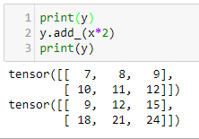
Here we have created two tensors, each with dimensions of 2 x 3. You can see that we have created a simple linear function (more about linear functions in Chapter 2, Deep Learning Fundamentals) and applied it to x and y and printed out the result. We can visualize this with the following diagram:

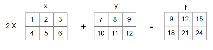
As you may know from linear algebra, matrix multiplication and addition occur element-wise so that for the first element of x, let's write this as X₀₀. This is multiplied by two and added to the first element of y, written as Y₀₀, giving F₀₀ = 9. X₀₁ = 2 and Y₀₁ = 8 so f₀₁ = 4 + 12. Notice that the indices start at zero.

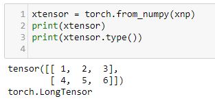
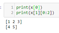
If you have never seen any linear algebra, don't worry too much about this, as we are going to brush up on these concepts in Chapter 2, Deep Learning Fundamentals, and you will get to practice with Python indexing shortly. For now, just consider our 2 x 3 tensors as tables with numbers in them.

There are many cases where we need to initialize torch tensors to default values. Here, we create three 2 x 3 tensors, filling them with zeros, ones, and random floating point numbers:

An important point to consider when we are initializing random arrays is the so-called seed of reproducibility. See what happens when you run the preceding code several times. You get a different array of random numbers each time. Often in machine learning, we need to be able to reproduce results. We can achieve this by using a random seed. This is demonstrated in the following code:

Notice that when you run this code many times, the tensor values stay the same. If you remove the seed by deleting the first line, the tensor values will be different each time the code is run. It does not matter what number you use to seed the random number generator, as long as it is consistently, achieves reproducible results.

Converting a NumPy array is as simple as performing an operation on it with a torch tensor. The following code should make this clear:

We can see the result of the type torch tensor. In many cases, we can use NumPy arrays interchangeably with tensors and always be sure the result is a tensor. However, there are times when we need to explicitly create a tensor from an array. This is done with the torch.from_numpy function:

To convert from a tensor to a NumPy array, simply call the torch.numpy() function:

Notice that we use Python's built-in type() function, as in type(object), rather than the tensor.type() we used previously. The NumPy arrays do not have a type attribute. Another important thing to understand is that NumPy arrays and PyTorch tensors share the same memory space. For example, see what happens when we change a variables value as demonstrated by the following code:

Note also that when we print a tensor, it returns a tuple consisting of the tensor itself and also its dtype, or data type attribute. It's important here because there are certain dtype arrays that cannot be turned into tensors. For example, consider the following code:

This will generate an error message telling us that only supported dtype are able to be converted into tensors. Clearly, int8 is not one of these supported types. We can fix this by converting our int8 array to an int64 array before passing it to torch.from_numpy. We do this with the numpy.astype function, as the following code demonstrates:

It is also important to understand how numpy dtype arrays convert to torch dtype. In the previous example, numpy int32 converts to IntTensor. The following table lists the torch dtype and their numpy equivalents:

The default dtype for tensors is FloatTensor; however, we can specify a particular data type by using the tensor's dtype attribute. For an example, see the following code:

torch.Tensor have most of the attributes and functionality of NumPy. For example, we can slice and index tensors in the same way as NumPy arrays:

Here, we have printed out the first element of x, written as x₀, and in the second example, we have printed out a slice of the second element of x; in this case, x₁₁ and x₁₂.

If you have not come across slicing and indexing, you may want to look at this again. Note that indexing begins at 0, not 1, and we have kept our subscript notation consistent with this. Notice also that the slice [1][0:2] is the elements x₁₀ and x₁₁, inclusive. It excludes the ending index, index 2, specified in the slice.

We can can create a reshaped copy of an existing tensor using the view() function. The following are three examples:

It is pretty clear what (3,2) and (6,1) do, but what about the –1 in the first example? This is useful if you know how many columns you require, but do not know how many rows this will fit into. Indicating –1 here is telling PyTorch to calculate the number of rows required. Using it without another dimension simply creates a tensor of a single row. You could rewrite example two mentioned previously, as follows, if you did not know the input tensor's shape but know that it needs to have three rows:

An important operation is swapping axes or transposing. For a two-dimensional tensor, we a can use tensor.transpose(), passing it the axis we want to transpose. In this example, the original 2 x 3 tensor becomes a 3 x 2 tensor. The rows simply become the columns:

In PyTorch, transpose() can only swap two axes at once. We could use transpose in multiple steps; however, a more convenient way is to use permute(), passing it the axes we want to swap. The following example should make this clear:

When we are considering tensors in two dimensions, we can visualize them as flat tables. When we move to higher dimensions, this visual representation becomes impossible. We simply run out of spatial dimensions. Part of the magic of deep learning is that it does not matter much in terms of the mathematics involved. Real-world features are each encoded into a dimension of a data structure. So, we may be dealing with tensors of potentially thousands of dimensions. Although it might be disconcerting, most of the ideas that can be illustrated in two or three dimensions work just as well in higher dimensions.

It is important to understand the difference between in place and assignment operations. When, for example, we use transpose(x), a value is returned but the value of x does not change. In all the examples up until now, we have been performing operations by assignment. That is, we have been assigning a variable to the result of an operation, or simply printing it to the output, as in the preceding example. In either case, the original variable remains untouched. Alternatively, we may need to apply an operation in place. We can, of course, assign a variable to itself, such as in x = x.transpose(0,1); however, a more convenient way to do this is with in place operations. In general, in place operations in PyTorch have a trailing underscore. For an example, see the following code:

As another example, here is the linear function we started this chapter with using in place operations on y: