Exploring Jupyter Notebook

Now that we have our libraries installed, we're ready to get started with Jupyter Notebook. Jupyter Notebook is a really nice way of creating interactive code and widgets. It lets us create interactive presentations with live code and experiment, as we're doing here.

If everything is set up correctly using Anaconda, we should already have Jupyter installed. Let's go ahead and take a look at Jupyter Notebook now.

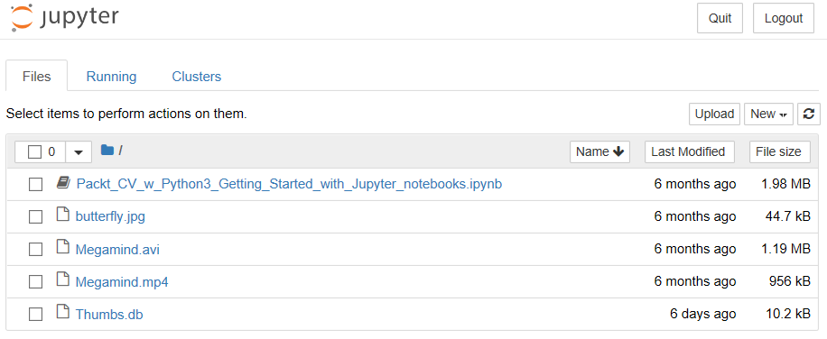
Open Command Prompt in the directory where your code files are, and then run the jupyter notebook command. This will open up a web browser in the directory where the command was executed. This should result in an interface that looks similar to the following screenshot:

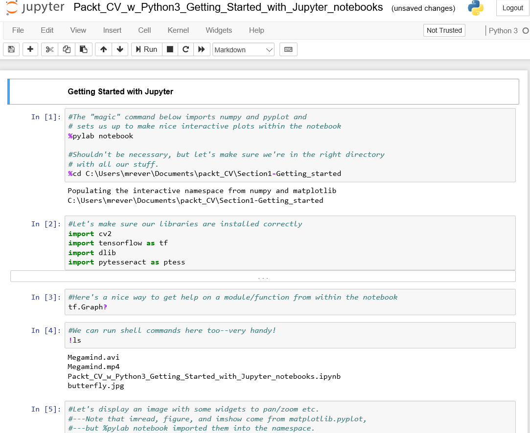
Next, open the .ipynb file so you can explore the basic functionalities of Jupyter Notebook. Once opened, we should see a page similar to the following screenshot:

As shown, there are blocks (called cells) where we can put in Python commands and Python code. We can also enter other commands, also known as magic commands, which are not part of Python per se, but allow us to do nice things within Jupyter or IPython (an interactive shell for Python). The % at the beginning means that the command is a magic command.

The biggest advantage here is that we can execute individual lines of code, instead of having to type out the entire code block in one go.

Let's go through some of the commands seen in the preceding screenshot, and see what they do, as follows:

1. The %pylab notebook command, as seen in the first cell, imports a lot of very useful and common libraries, particularly NumPy and PyPlot, without us needing to explicitly call the import commands. It also sets up a Notebook easily.
2. Also in the first cell, we assign the directory that we will be working from, as follows:

%cd C:\Users\<user_name>\Documents\<Folder_name>\Section1-Getting_started

This results in the following output:

So far, so good!

3. The following cell shows how to import our libraries. We're going to import OpenCV, TensorFlow, dlib, and Tesseract, just to make sure that everything is working and that there aren't any nasty surprises. This is done using the following code block:

import cv2
import tensorflow as tf
import dlib
import pytesseract as ptess

If you get an error message here, redo the installation of the libraries, following the instructions carefully. Sometimes things do go wrong, depending on our system.

4. The third cell in the screenshot contains the command for importing the graph module in TensorFlow. This can come in handy for getting help on a function from within the Notebook, as follows:

tf.Graph?

We will discuss this function in Chapter 7, Deep Learning Image Classification with TensorFlow.

5. Another neat thing about Jupyter Notebooks is that we can run shell commands right in the cell. As seen in the fourth cell in the screenshot (repeated here), the ls command shows us all the files in the directory we are working from:

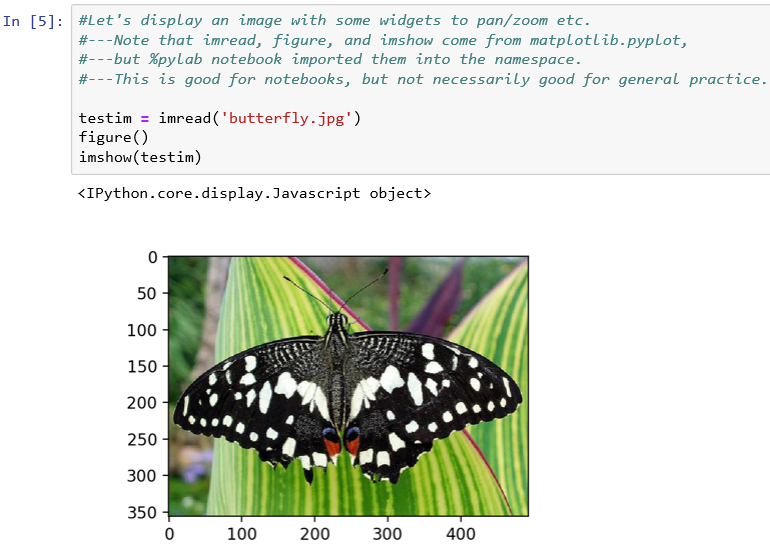
6. In this book, we'll be working with a lot of images, so we'll want to see the images right in the Notebook. Use the imread() function to read the image file from your directory. After that, your next step is to create a figure() widget to display the image. Finally, use the imshow() function to actually display the image.

This entire process is summarized in the following screenshot:

This is awesome, because we have widgets that are flexible.

7. By grabbing the bottom-right corner, we can shrink this to a reasonable size to see our color image with pixel axes displayed. We also have the pan option available. By clicking on it, we can pan our image and box zoom it. Hitting the home button resets the original view.

We will want take a look at our images, and processed images and so forth—as seen previously, this is a very handy and simple way to do it. We can also use PyLab inline, which is useful for certain things, as we'll see.

8. As we know, part of computer vision is working with videos. To play videos within the notebook, we need to import some libraries and use IPython's HTML capability, as shown in the following screenshot:

Essentially, we're using our web browser's capability to play back videos. So, it's not really Python that's doing it, but our web browser, which enables interactivity between Jupyter Notebook and our browser.

Here, we defined the playvideo() function, which takes the video filename as an input and returns an HTML object with our video.

9. Execute the following command on Jupyter to play the Megamind video. It's just a clip of the movie Megamind, which (for some reason) comes with OpenCV if we download all the source code:

playvideo(' ./Megamind.mp4')

10. You will see a black box, and if you scroll down, you'll find a play button. Hit this and the movie will play, as seen in the following screenshot:

This can be used to play our own videos. All you have to do is point the command to the video that you want to play.

Once you have all this running, you should be in good shape to run the projects that we're going to take a look at in the coming chapters.