Your first network in NetworkX

Now, let's create and visualize a small network using NetworkX! For the code in this book, you will need Python 3.4 or higher and NetworkX 2.2 or greater. I also highly recommend Jupyter Lab as an interactive Python environment. The code in this book is available as Jupyter notebooks at https://github.com/PacktPublishing/Network-Science-with-Python-and-NetworkX-Quick-Start-Guide.

The following example creates an undirected, unweighted network, adds edges and nodes, and then generates a visualization. Other types of networks will be discussed in Chapter 2, Working with Networks in NetworkX. First, we import the networkx package. In this book, I will use the convention of importing the library with the alias nx:

import networkx as nx

Next, we create a Graph object, representing an undirected network, given as follows:

G = nx.Graph()

Now that the graph exists, we can add nodes one at a time with the add_node() method, or all at once with add_nodes_from(). When adding nodes to a network, each node has to have a unique ID. The ID can be a number, a string, or a tuple. In fact, you can use any Python object as an ID, as long as it has a __hash__() method defined. For this example, we'll use letters as node IDs, shown as follows:

G.add_node('A')
G.add_nodes_from(['B', 'C'])

Similarly, edges can be added one at a time with add_edge(), or all at once with add_edges_from(), shown as follows:

G.add_edge('A', 'B')
G.add_edges_from([('B', 'C'), ('A', 'C')])

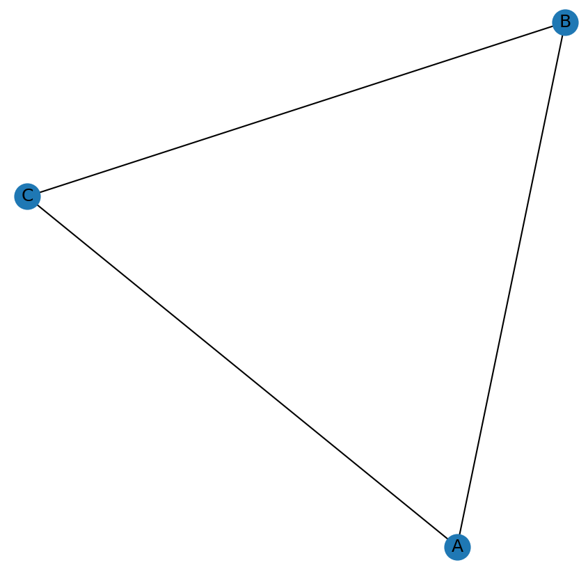
So far, the A, B, and C nodes, as well as the edges connecting them, have been added. The following code draws a simple visualization of the network:

plt.figure(figsize=(7.5, 7.5))
nx.draw_networkx(G)
plt.show()

In the preceding code, figure() is used to create a 7.5 by 7.5 inch figure, which will hold the visualization. The draw_networkx() function uses the Graph object G to produce a visualization. The show() function renders the visualization, but can be omitted if you are running the examples in Jupyter Lab. The visualization should appear similar to the following:

Your visualization may look slightly different from the one shown previously. This is because visualizations in NetworkX sometimes use randomized algorithms. The randomized algorithms can be configured to produce the same output each time by setting the random seed. The following code sets the random seeds used by NetworkX (this code will also appear at the beginning of the example code for all future chapters):

import random
from numpy import random as nprand
seed = hash("Network Science in Python") % 2**32
nprand.seed(seed)
random.seed(seed)

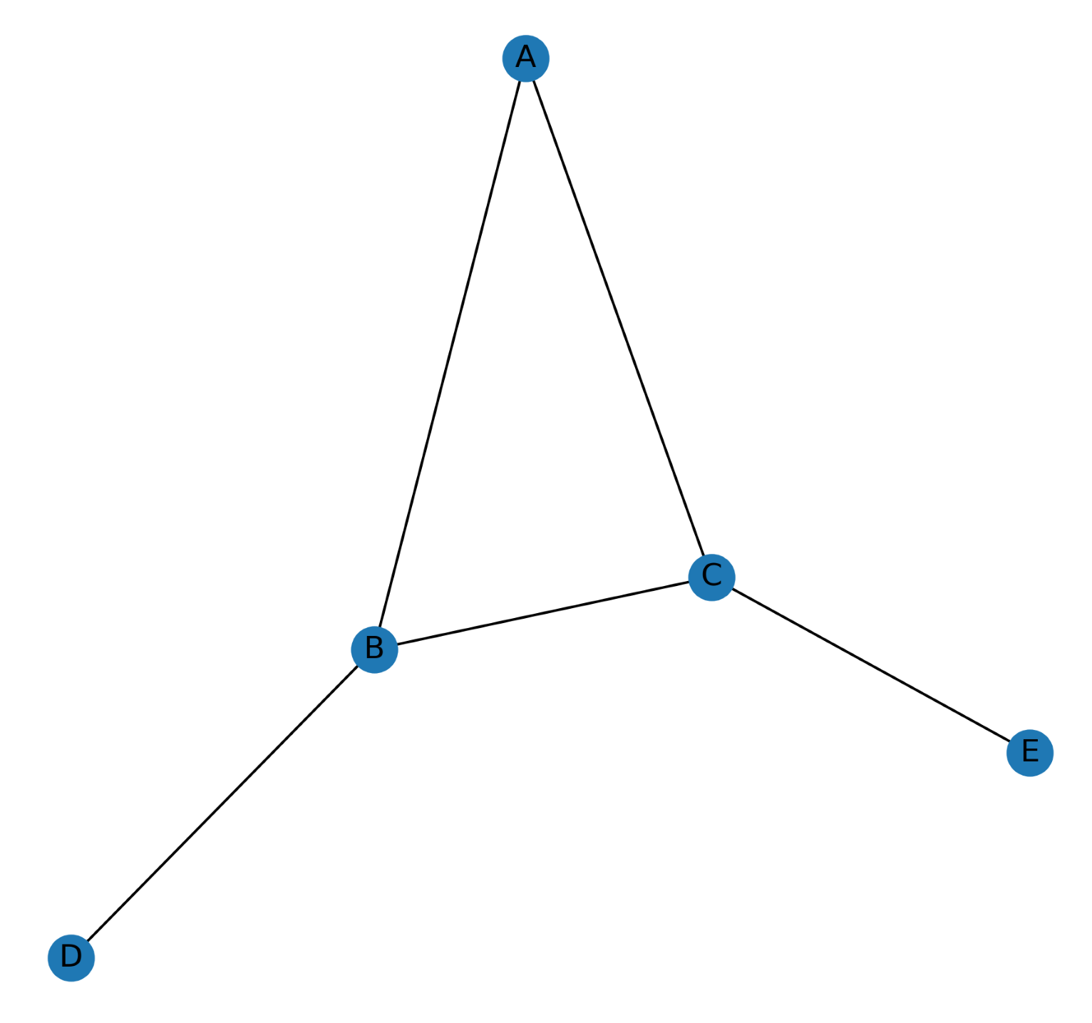
Nodes can also be added using a nifty shortcut. If you try to add an edge referring to a node ID that isn't in the network, NetworkX will automatically add the node! So, in practice, you won't often need to call add_node() directly. The following code adds nodes and edges so that the network matches the example network from earlier and creates a new visualization:

G.add_edges_from([('B', 'D'), ('C', 'E')]) 
nx.draw_networkx(G)

The draw_networkx() function now produces a visualization including the new D and E nodes: