Implementing loss functions

For this recipe, we will cover some of the main loss functions that we can use in TensorFlow. Loss functions are a key aspect of machine learning algorithms. They measure the distance between the model outputs and the target (truth) values.

In order to optimize our machine learning algorithms, we will need to evaluate the outcomes. Evaluating outcomes in TensorFlow depends on specifying a loss function. A loss function tells TensorFlow how good or bad the predictions are compared to the desired result. In most cases, we will have a set of data and a target on which to train our algorithm. The loss function compares the target to the prediction (it measures the distance between the model outputs and the target truth values) and provides a numerical quantification between the two.

Getting ready

We will first start a computational graph and load matplotlib, a Python plotting package, as follows:

import matplotlib.pyplot as plt 
import TensorFlow as tf 

Now that we are ready to plot, let's proceed to the recipe without further ado.

How to do it...

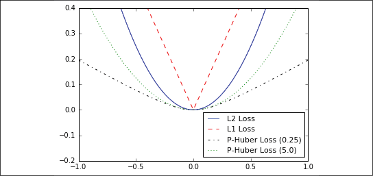
First, we will talk about loss functions for regression, which means predicting a continuous dependent variable. To start, we will create a sequence of our predictions and a target as a tensor. We will output the results across 500 x values between -1 and 1. See the How it works... section for a plot of the outputs. Use the following code:

x_vals = tf.linspace(-1., 1., 500) 
target = tf.constant(0.) 

The L2 norm loss is also known as the Euclidean loss function. It is just the square of the distance to the target. Here, we will compute the loss function as if the target is zero. The L2 norm is a great loss function because it is very curved near the target and algorithms can use this fact to converge to the target more slowly the closer it gets to zero. We can implement this as follows:

def l2(y_true, y_pred):
    return tf.square(y_true - y_pred) 

The L1 norm loss is also known as the absolute loss function. Instead of squaring the difference, we take the absolute value. The L1 norm is better for outliers than the L2 norm because it is not as steep for larger values. One issue to be aware of is that the L1 norm is not smooth at the target, and this can result in algorithms not converging well. It appears as follows:

def l1(y_true, y_pred):
    return tf.abs(y_true - y_pred)

Pseudo-Huber loss is a continuous and smooth approximation to the Huber loss function. This loss function attempts to take the best of the L1 and L2 norms by being convex near the target and less steep for extreme values. The form depends on an extra parameter, delta, which dictates how steep it will be. We will plot two forms, delta1 = 0.25 and delta2 = 5, to show the difference, as follows:

def phuber1(y_true, y_pred):
    delta1 = tf.constant(0.25) 
    return tf.multiply(tf.square(delta1), tf.sqrt(1. +  
                        tf.square((y_true - y_pred)/delta1)) - 1.) 
def phuber2(y_true, y_pred):
    delta2 = tf.constant(5.) 
    return tf.multiply(tf.square(delta2), tf.sqrt(1. +  
                        tf.square((y_true - y_pred)/delta2)) - 1.) 

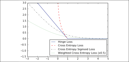
Now, we'll move on to loss functions for classification problems. Classification loss functions are used to evaluate loss when predicting categorical outcomes. Usually, the output of our model for a class category is a real-value number between 0 and 1. Then, we choose a cutoff (0.5 is commonly chosen) and classify the outcome as being in that category if the number is above the cutoff. Next, we'll consider various loss functions for categorical outputs.

To start, we will need to redefine our predictions (x_vals) and target. We will save the outputs and plot them in the next section. Use the following:

x_vals = tf.linspace(-3., 5., 500) 
target = tf.fill([500,], 1.)

Hinge loss is mostly used for support vector machines but can be used in neural networks as well. It is meant to compute a loss among two target classes, 1 and -1. In the following code, we are using the target value 1, so the closer our predictions are to 1, the lower the loss value:

def hinge(y_true, y_pred):
    return tf.maximum(0., 1. - tf.multiply(y_true, y_pred))

Cross-entropy loss for a binary case is also sometimes referred to as the logistic loss function. It comes about when we are predicting the two classes 0 or 1. We wish to measure a distance from the actual class (0 or 1) to the predicted value, which is usually a real number between 0 and 1. To measure this distance, we can use the cross-entropy formula from information theory, as follows:

def xentropy(y_true, y_pred):
    return (- tf.multiply(y_true, tf.math.log(y_pred)) -   
          tf.multiply((1. - y_true), tf.math.log(1. - y_pred))) 

Sigmoid cross-entropy loss is very similar to the previous loss function except we transform the x values using the sigmoid function before we put them in the cross-entropy loss, as follows:

def xentropy_sigmoid(y_true, y_pred):
    return tf.nn.sigmoid_cross_entropy_with_logits(labels=y_true,  
                                                   logits=y_pred) 

Weighted cross-entropy loss is a weighted version of sigmoid cross-entropy loss. We provide a weight on the positive target. For an example, we will weight the positive target by 0.5, as follows:

def xentropy_weighted(y_true, y_pred):
    weight = tf.constant(0.5) 
    return tf.nn.weighted_cross_entropy_with_logits(labels=y_true,
                                                    logits=y_pred,  
                                                pos_weight=weight)

Softmax cross-entropy loss operates on non-normalized outputs. This function is used to measure a loss when there is only one target category instead of multiple. Because of this, the function transforms the outputs into a probability distribution via the softmax function and then computes the loss function from a true probability distribution, as follows:

def softmax_xentropy(y_true, y_pred):
    return tf.nn.softmax_cross_entropy_with_logits(labels=y_true,                                                    logits=y_pred)
    
unscaled_logits = tf.constant([[1., -3., 10.]]) 
target_dist = tf.constant([[0.1, 0.02, 0.88]])
print(softmax_xentropy(y_true=target_dist,                        y_pred=unscaled_logits))
[ 1.16012561] 

Sparse softmax cross-entropy loss is almost the same as softmax cross-entropy loss, except instead of the target being a probability distribution, it is an index of which category is true. Instead of a sparse all-zero target vector with one value of 1, we just pass in the index of the category that is the true value, as follows:

def sparse_xentropy(y_true, y_pred):
    return tf.nn.sparse_softmax_cross_entropy_with_logits(
                                                    labels=y_true,
                                                    logits=y_pred) 
unscaled_logits = tf.constant([[1., -3., 10.]]) 
sparse_target_dist = tf.constant([2]) 
print(sparse_xentropy(y_true=sparse_target_dist,  
                      y_pred=unscaled_logits))
[ 0.00012564] 

Now let's understand better how such loss functions operate by plotting them on a graph.

How it works...

Here is how to use matplotlib to plot the regression loss functions:

x_vals = tf.linspace(-1., 1., 500) 
target = tf.constant(0.) 
funcs = [(l2, 'b-', 'L2 Loss'),
         (l1, 'r--', 'L1 Loss'),
         (phuber1, 'k-.', 'P-Huber Loss (0.25)'),
         (phuber2, 'g:', 'P-Huber Loss (5.0)')]
for func, line_type, func_name in funcs:
    plt.plot(x_vals, func(y_true=target, y_pred=x_vals), 
             line_type, label=func_name)
plt.ylim(-0.2, 0.4) 
plt.legend(loc='lower right', prop={'size': 11}) 
plt.show()

We get the following plot as output from the preceding code:

Figure 2.1: Plotting various regression loss functions

Here is how to use matplotlib to plot the various classification loss functions:

x_vals = tf.linspace(-3., 5., 500)  
target = tf.fill([500,], 1.)
funcs = [(hinge, 'b-', 'Hinge Loss'),
         (xentropy, 'r--', 'Cross Entropy Loss'),
         (xentropy_sigmoid, 'k-.', 'Cross Entropy Sigmoid Loss'),
         (xentropy_weighted, 'g:', 'Weighted Cross Enropy Loss            (x0.5)')]
for func, line_type, func_name in funcs:
    plt.plot(x_vals, func(y_true=target, y_pred=x_vals), 
             line_type, label=func_name)
plt.ylim(-1.5, 3) 
plt.legend(loc='lower right', prop={'size': 11}) 
plt.show()

We get the following plot from the preceding code:

Figure 2.2: Plots of classification loss functions

Each of these loss curves provides different advantages to the neural network optimizing it. We are now going to discuss this a little bit more.

There's more...

Here is a table summarizing the properties and benefits of the different loss functions that we have just graphically described:

The remaining classification loss functions all have to do with the type of cross-entropy loss. The cross-entropy sigmoid loss function is for use on unscaled logits and is preferred over computing the sigmoid loss and then the cross-entropy loss, because TensorFlow has better built-in ways to handle numerical edge cases. The same goes for softmax cross-entropy and sparse softmax cross-entropy.

There are also many other metrics to look at when evaluating a model. Here is a list of some more to consider:

In your choice of the right metric, you have to both evaluate the problem you have to solve (because each metric will behave differently and, depending on the problem at hand, some loss minimization strategies will prove better than others for our problem), and to experiment with the behavior of the neural network.