

Combining everything together
In this section, we will combine everything we have illustrated so far and create a classifier for the iris dataset. The iris dataset is described in more detail in the Working with data sources recipe in Chapter 1, Getting Started with TensorFlow. We will load this data and make a simple binary classifier to predict whether a flower is the species Iris setosa or not. To be clear, this dataset has three species, but we will only predict whether a flower is a single species, Iris setosa or not, giving us a binary classifier.
Getting ready
We will start by loading the libraries and data and then transform the target accordingly. First, we load the libraries needed for our recipe. For the Iris dataset, we need the TensorFlow Datasets module, which we haven't used before in our recipes. Note that we also load matplotlib here, because we would like to plot the resultant line afterward:
import matplotlib.pyplot as plt
import NumPy as np
import TensorFlow as tf
import TensorFlow_datasets as tfds
How to do it...
As a starting point, let's first declare our batch size using a global variable:
batch_size = 20
Next, we load the iris data. We will also need to transform the target data to be just 1 or 0, whether the target is setosa or not. Since the iris dataset marks setosa as a 0, we will change all targets with the value 0 to 1, and the other values all to 0. We will also only use two features, petal length and petal width. These two features are the third and fourth entry in each row of the dataset:
iris = tfds.load('iris', split='train[:90%]', W)
iris_test = tfds.load('iris', split='train[90%:]', as_supervised=True)
def iris2d(features, label):
    return features[2:], tf.cast((label == 0), dtype=tf.float32)
train_generator = (iris
                   .map(iris2d)
                   .shuffle(buffer_size=100)
                   .batch(batch_size)
                  )
test_generator = iris_test.map(iris2d).batch(1)
As shown in the previous chapter, we use the TensorFlow dataset functions to both load and operate the necessary transformations by creating a data generator that can dynamically feed our network with data, instead of keeping it in an in-memory NumPy matrix. As a first step, we load the data, specifying that we want to split it (using the parameters split='train[:90%]' and split='train[90%:]'). This allows us to reserve a part (10%) of the dataset for the model evaluation, using data that has not been part of the training phase.
We also specify the parameter, as_supervised=True, that will allow us to access the data as tuples of features and labels when iterating from the dataset.
Now we transform the dataset into an iterable generator by applying successive transformations. We shuffle the data, we define the batch to be returned by the iterable, and, most important, we apply a custom function that filters and transforms the features and labels returned from the dataset at the same time.
Then, we define the linear model. The model will take the usual form bX+a. Remember that TensorFlow has loss functions with the sigmoid built in, so we just need to define the output of the model prior to the sigmoid function:
def linear_model(X, A, b):
    my_output = tf.add(tf.matmul(X, A), b)
    return tf.squeeze(my_output)
Now, we add our sigmoid cross-entropy loss function with TensorFlow's built-in sigmoid_cross_entropy_with_logits() function:
def xentropy(y_true, y_pred):
    return tf.reduce_mean(
        tf.nn.sigmoid_cross_entropy_with_logits(labels=y_true,
                                                logits=y_pred))
We also have to tell TensorFlow how to optimize our computational graph by declaring an optimizing method. We will want to minimize the cross-entropy loss. We will also choose 0.02 as our learning rate:
my_opt = tf.optimizers.SGD(learning_rate=0.02)
Now, we will train our linear model with 300 iterations. We will feed in the three data points that we require: petal length, petal width, and the target variable. Every 30 iterations, we will print the variable values:
tf.random.set_seed(1)
np.random.seed(0)
A = tf.Variable(tf.random.normal(shape=[2, 1]))
b = tf.Variable(tf.random.normal(shape=[1]))
history = list()
for i in range(300):
    iteration_loss = list()
    for features, label in train_generator:
        with tf.GradientTape() as tape:
            predictions = linear_model(features, A, b)
            loss = xentropy(label, predictions)
        iteration_loss.append(loss.NumPy())
        gradients = tape.gradient(loss, [A, b])
        my_opt.apply_gradients(zip(gradients, [A, b]))
    history.append(np.mean(iteration_loss))
    if (i + 1) % 30 == 0:
        print(f'Step # {i+1} Weights: {A.NumPy().T} \
              Biases: {b.NumPy()}')
        print(f'Loss = {loss.NumPy()}')
Step # 30 Weights: [[-1.1206311  1.2985772]] Biases: [1.0116111]
Loss = 0.4503694772720337
…
Step # 300 Weights: [[-1.5611029   0.11102282]] Biases: [3.6908474]
Loss = 0.10326375812292099
If we plot the loss against the iterations, we can acknowledge from the smoothness of the reduction of the loss over time how the learning has been quite an easy task for the linear model:
plt.plot(history)
plt.xlabel('iterations')
plt.ylabel('loss')
plt.show()
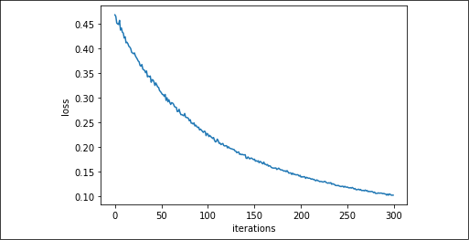
Figure 2.8: Cross-entropy error for the Iris setosa data
We'll conclude by checking the performance on our reserved test data. This time we just take the examples from the test dataset. As expected, the resulting cross-entropy value is analogous to the training one:
predictions = list()
labels = list()
for features, label in test_generator:
    predictions.append(linear_model(features, A, b).NumPy())
    labels.append(label.NumPy()[0])

test_loss = xentropy(np.array(labels), np.array(predictions)).NumPy()
print(f"test cross-entropy is {test_loss}")
test cross-entropy is 0.10227929800748825
The next set of commands extracts the model variables and plots the line on a graph:
coefficients = np.ravel(A.NumPy())
intercept = b.NumPy()
# Plotting batches of examples
for j, (features, label) in enumerate(train_generator):
    setosa_mask = label.NumPy() == 1
    setosa = features.NumPy()[setosa_mask]
    non_setosa = features.NumPy()[~setosa_mask]
    plt.scatter(setosa[:,0], setosa[:,1], c='red', label='setosa')
    plt.scatter(non_setosa[:,0], non_setosa[:,1], c='blue', label='Non-setosa')
    if j==0:
        plt.legend(loc='lower right')
# Computing and plotting the decision function
a = -coefficients[0] / coefficients[1]
xx = np.linspace(plt.xlim()[0], plt.xlim()[1], num=10000)
yy = a * xx - intercept / coefficients[1]
on_the_plot = (yy > plt.ylim()[0]) & (yy < plt.ylim()[1])
plt.plot(xx[on_the_plot], yy[on_the_plot], 'k--')
plt.xlabel('Petal Length')
plt.ylabel('Petal Width')
plt.show()
The resultant graph is in the How it works... section, where we also discuss the validity and reproducibility of the obtained results.
How it works...
Our goal was to fit a line between the Iris setosa points and the other two species using only petal width and petal length. If we plot the points, and separate the area of the plot where classifications are zero from the area where classifications are one with a line, we see that we have achieved this:
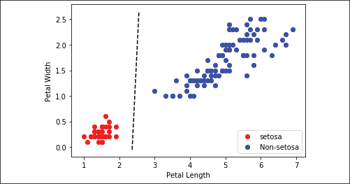
Figure 2.9: Plot of Iris setosa and non-setosa for petal width versus petal length; the solid line is the linear separator that we achieved after 300 iterations
The way the separating line is defined depends on the data, the network architecture, and the learning process. Different starting situations, even due to the random initialization of the neural network's weights, may provide you with a slightly different solution.
There's more...
While we achieved our objective of separating the two classes with a line, it may not be the best model for separating two classes. For instance, after adding new observations, we may realize that our solution badly separates the two classes. As we progress into the next chapter, we will start dealing with recipes that address these problems by providing testing, randomization, and specialized layers that will increase the generalization capabilities of our recipes.
See also
- For information about the Iris dataset, see the documentation at https://archive.ics.uci.edu/ml/datasets/iris.
- If you want to understand more about decision boundaries drawing for machine learning algorithms, we warmly suggest this excellent Medium article from Navoneel Chakrabarty: https://towardsdatascience.com/decision-boundary-visualization-a-z-6a63ae9cca7d