Working with batch and stochastic training

While TensorFlow updates our model variables according to backpropagation, it can operate on anything from a one-datum observation (as we did in the previous recipe) to a large batch of data at once. Operating on one training example can make for a very erratic learning process, while using too large a batch can be computationally expensive. Choosing the right type of training is crucial for getting our machine learning algorithms to converge to a solution.

Getting ready

In order for TensorFlow to compute the variable gradients for backpropagation to work, we have to measure the loss on a sample or multiple samples. Stochastic training only works on one randomly sampled data-target pair at a time, just as we did in the previous recipe. Another option is to put a larger portion of the training examples in at a time and average the loss for the gradient calculation. The sizes of the training batch can vary, up to and including the whole dataset at once. Here, we will show how to extend the prior regression example, which used stochastic training, to batch training.

We will start by loading NumPy, matplotlib, and TensorFlow, as follows:

import matplotlib as plt 
import NumPy as np 
import TensorFlow as tf 

Now we just have to script our code and test our recipe in the How to do it… section.

How to do it...

We start by declaring a batch size. This will be how many data observations we will feed through the computational graph at one time:

batch_size = 20

Next, we just apply small modifications to the code used before for the regression problem:

np.random.seed(0)
x_vals = np.random.normal(1, 0.1, 100).astype(np.float32) 
y_vals = (x_vals * (np.random.normal(1, 0.05, 100) - 0.5)).astype(np.float32)
def loss_func(y_true, y_pred):
    return tf.reduce_mean(tf.square(y_pred - y_true))
tf.random.set_seed(1)
np.random.seed(0)
weights = tf.Variable(tf.random.normal(shape=[1])) 
biases = tf.Variable(tf.random.normal(shape=[1])) 
history_batch = list()
for i in range(50):    
    rand_index = np.random.choice(100, size=batch_size) 
    rand_x = [x_vals[rand_index]] 
    rand_y = [y_vals[rand_index]]
    with tf.GradientTape() as tape:
        predictions = my_output(rand_x, weights, biases)
        loss = loss_func(rand_y, predictions)
    history_batch.append(loss.NumPy())
    gradients = tape.gradient(loss, [weights, biases])
    my_opt.apply_gradients(zip(gradients, [weights, biases]))
    if (i + 1) % 25 == 0: 
        print(f'Step # {i+1} Weights: {weights.NumPy()} \
              Biases: {biases.NumPy()}')
        print(f'Loss = {loss.NumPy()}')

Since our previous recipe, we have learned how to use matrix multiplication in our network and in our cost function. At this point, we just need to deal with inputs that are made of more rows as batches instead of single examples. We can even compare it with the previous approach, which we can now name stochastic optimization:

tf.random.set_seed(1)
np.random.seed(0)
weights = tf.Variable(tf.random.normal(shape=[1])) 
biases = tf.Variable(tf.random.normal(shape=[1])) 
history_stochastic = list()
for i in range(50):    
    rand_index = np.random.choice(100, size=1) 
    rand_x = [x_vals[rand_index]] 
    rand_y = [y_vals[rand_index]]
    with tf.GradientTape() as tape:
        predictions = my_output(rand_x, weights, biases)
        loss = loss_func(rand_y, predictions)
    history_stochastic.append(loss.NumPy())
    gradients = tape.gradient(loss, [weights, biases])
    my_opt.apply_gradients(zip(gradients, [weights, biases]))
    if (i + 1) % 25 == 0: 
        print(f'Step # {i+1} Weights: {weights.NumPy()} \
              Biases: {biases.NumPy()}')
        print(f'Loss = {loss.NumPy()}')

Just running the code will retrain our network using batches. At this point, we need to evaluate the results, get some intuition about how it works, and reflect on the results. Let's proceed to the next section.

How it works...

Batch training and stochastic training differ in their optimization methods and their convergence. Finding a good batch size can be difficult. To see how convergence differs between batch training and stochastic training, you are encouraged to change the batch size to various levels.

A visual comparison of the two approaches will explain better how using batches for this problem resulted in the same optimization as stochastic training, though there were fewer fluctuations during the process. Here is the code to produce the plot of both the stochastic and batch losses for the same regression problem. Note that the batch loss is much smoother and the stochastic loss is much more erratic:

plt.plot(history_stochastic, 'b-', label='Stochastic Loss') 
plt.plot(history_batch, 'r--', label='Batch Loss') 
plt.legend(loc='upper right', prop={'size': 11}) 
plt.show() 

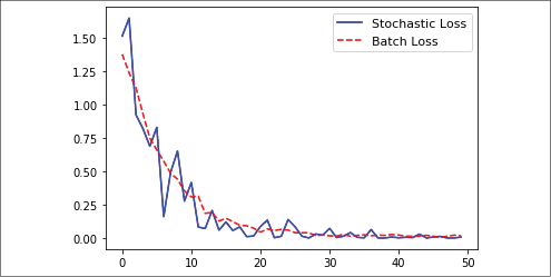
Figure 2.7: Comparison of L2 loss when using stochastic and batch optimization

Now our graph displays a smoother trend line. The persistent presence of bumps could be solved by reducing the learning rate and adjusting the batch size.

There's more...