Implementing backpropagation

One of the benefits of using TensorFlow is that it can keep track of operations and automatically update model variables based on backpropagation. In this recipe, we will introduce how to use this aspect to our advantage when training machine learning models.

Getting ready

Now, we will introduce how to change our variables in the model in such a way that a loss function is minimized. We have learned how to use objects and operations, and how to create loss functions that will measure the distance between our predictions and targets. Now, we just have to tell TensorFlow how to backpropagate errors through our network in order to update the variables in such a way to minimize the loss function. This is achieved by declaring an optimization function. Once we have an optimization function declared, TensorFlow will go through and figure out the backpropagation terms for all of our computations in the graph. When we feed data in and minimize the loss function, TensorFlow will modify our variables in the network accordingly.

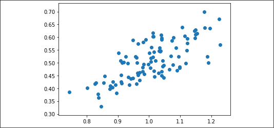
For this recipe, we will do a very simple regression algorithm. We will sample random numbers from a normal distribution, with mean 1 and standard deviation 0.1. Then, we will run the numbers through one operation, which will be to multiply them by a weight tensor and then adding a bias tensor. From this, the loss function will be the L2 norm between the output and the target. Our target will show a high correlation with our input, so the task won't be too complex, yet the recipe will be interestingly demonstrative, and easily reusable for more complex problems.

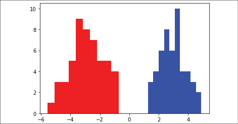
The second example is a very simple binary classification algorithm. Here, we will generate 100 numbers from two normal distributions, N(-3,1) and N(3,1). All the numbers from N(-3, 1) will be in target class 0, and all the numbers from N(3, 1) will be in target class 1. The model to differentiate these classes (which are perfectly separable) will again be a linear model optimized accordingly to the sigmoid cross-entropy loss function, thus, at first operating a sigmoid transformation on the model result and then computing the cross-entropy loss function.

While specifying a good learning rate helps the convergence of algorithms, we must also specify a type of optimization. From the preceding two examples, we are using standard gradient descent. This is implemented with the tf.optimizers.SGD TensorFlow function.

How to do it...

We'll start with the regression example. First, we load the usual numerical Python packages that always accompany our recipes, NumPy and TensorFlow:

import NumPy as np 
import TensorFlow as tf 

Next, we create the data. In order to make everything easily replicable, we want to set the random seed to a specific value. We will always repeat this in our recipes, so we exactly obtain the same results; check yourself how chance may vary the results in the recipes, by simply changing the seed number.

Moreover, in order to get assurance that the target and input have a good correlation, plot a scatterplot of the two variables:

np.random.seed(0)
x_vals = np.random.normal(1, 0.1, 100).astype(np.float32) 
y_vals = (x_vals * (np.random.normal(1, 0.05, 100) - 0.5)).astype(np.float32)
plt.scatter(x_vals, y_vals)
plt.show()

Figure 2.3: Scatterplot of x_vals and y_vals

We add the structure of the network (a linear model of the type bX + a) as a function:

def my_output(X, weights, biases):
    return tf.add(tf.multiply(X, weights), biases)

Next, we add our L2 Loss function to be applied to the results of the network:

def loss_func(y_true, y_pred):
    return tf.reduce_mean(tf.square(y_pred - y_true))

Now, we have to declare a way to optimize the variables in our graph. We declare an optimization algorithm. Most optimization algorithms need to know how far to step in each iteration. Such a distance is controlled by the learning rate. Setting it to a correct value is specific to the problem we are dealing with, so we can figure out a suitable setting only by experimenting. Anyway, if our learning rate is too high, our algorithm might overshoot the minimum, but if our learning rate is too low, our algorithm might take too long to converge.

The learning rate has a big influence on convergence and we will discuss it again at the end of the section. While we're using the standard gradient descent algorithm, there are many other alternative options. There are, for instance, optimization algorithms that operate differently and can achieve a better or worse optimum depending on the problem. For a great overview of different optimization algorithms, see the paper by Sebastian Ruder in the See also section at the end of this recipe:

my_opt = tf.optimizers.SGD(learning_rate=0.02)

Now we can initialize our network variables (weights and biases) and set a recording list (named history) to help us visualize the optimization steps:

tf.random.set_seed(1)
np.random.seed(0)
weights = tf.Variable(tf.random.normal(shape=[1])) 
biases = tf.Variable(tf.random.normal(shape=[1])) 
history = list()

The final step is to loop through our training algorithm and tell TensorFlow to train many times. We will do this 100 times and print out results every 25^th iteration. To train, we will select a random x and y entry and feed it through the graph. TensorFlow will automatically compute the loss, and slightly change the weights and biases to minimize the loss:

for i in range(100): 
    rand_index = np.random.choice(100) 
    rand_x = [x_vals[rand_index]] 
    rand_y = [y_vals[rand_index]]
    with tf.GradientTape() as tape:
        predictions = my_output(rand_x, weights, biases)
        loss = loss_func(rand_y, predictions)
    history.append(loss.NumPy())
    gradients = tape.gradient(loss, [weights, biases])
    my_opt.apply_gradients(zip(gradients, [weights, biases]))
    if (i + 1) % 25 == 0: 
        print(f'Step # {i+1} Weights: {weights.NumPy()} Biases: {biases.NumPy()}')
        print(f'Loss = {loss.NumPy()}') 
Step # 25 Weights: [-0.58009654] Biases: [0.91217995]
Loss = 0.13842473924160004
Step # 50 Weights: [-0.5050226] Biases: [0.9813488]
Loss = 0.006441597361117601
Step # 75 Weights: [-0.4791306] Biases: [0.9942327]
Loss = 0.01728087291121483
Step # 100 Weights: [-0.4777394] Biases: [0.9807473]
Loss = 0.05371852591633797

In the loops, tf.GradientTape() allows TensorFlow to track the computations and calculate the gradient with respect to the observed variables. Every variable that is within the GradientTape() scope is monitored (please keep in mind that constants are not monitored, unless you explicitly state it with the command tape.watch(constant)). Once you've completed the monitoring, you can compute the gradient of a target in respect of a list of sources (using the command tape.gradient(target, sources)) and get back an eager tensor of the gradients that you can apply to the minimization process. The operation is automatically concluded with the updating of your sources (in our case, the weights and biases variables) with new values.

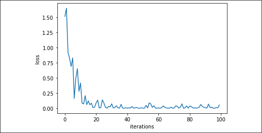
When the training is completed, we can visualize how the optimization process operates over successive gradient applications:

plt.plot(history)
plt.xlabel('iterations')
plt.ylabel('loss')
plt.show()

Figure 2.4: L2 loss through iterations in our recipe

At this point, we will introduce the code for the simple classification example. We can use the same TensorFlow script, with some updates. Remember, we will attempt to find an optimal set of weights and biases that will separate the data into two different classes.

First, we pull in the data from two different normal distributions, N(-3, 1) and N(3, 1). We will also generate the target labels and visualize how the two classes are distributed along our predictor variable:

np.random.seed(0)
x_vals = np.concatenate((np.random.normal(-3, 1, 50), 
                         np.random.normal(3, 1, 50))
                    ).astype(np.float32) 
y_vals = np.concatenate((np.repeat(0., 50), np.repeat(1., 50))).astype(np.float32) 
plt.hist(x_vals[y_vals==1], color='b')
plt.hist(x_vals[y_vals==0], color='r')
plt.show()

Figure 2.5: Class distribution on x_vals

Because the specific loss function for this problem is sigmoid cross-entropy, we update our loss function:

def loss_func(y_true, y_pred):
    return tf.reduce_mean(
        tf.nn.sigmoid_cross_entropy_with_logits(labels=y_true, 
                                                logits=y_pred))

Next, we initialize our variables:

tf.random.set_seed(1)
np.random.seed(0)
weights = tf.Variable(tf.random.normal(shape=[1])) 
biases = tf.Variable(tf.random.normal(shape=[1])) 
history = list()

Finally, we loop through a randomly selected data point several hundred times and update the weights and biases variables accordingly. As we did before, every 25 iterations we will print out the value of our variables and the loss:

for i in range(100):    
    rand_index = np.random.choice(100) 
    rand_x = [x_vals[rand_index]] 
    rand_y = [y_vals[rand_index]]
    with tf.GradientTape() as tape:
        predictions = my_output(rand_x, weights, biases)
        loss = loss_func(rand_y, predictions)
    history.append(loss.NumPy())
    gradients = tape.gradient(loss, [weights, biases])
    my_opt.apply_gradients(zip(gradients, [weights, biases]))
    if (i + 1) % 25 == 0: 
        print(f'Step {i+1} Weights: {weights.NumPy()} Biases: {biases.NumPy()}')
        print(f'Loss = {loss.NumPy()}')
Step # 25 Weights: [-0.01804185] Biases: [0.44081175]
Loss = 0.5967269539833069
Step # 50 Weights: [0.49321094] Biases: [0.37732077]
Loss = 0.3199256658554077
Step # 75 Weights: [0.7071932] Biases: [0.32154965]
Loss = 0.03642747551202774
Step # 100 Weights: [0.8395616] Biases: [0.30409005]
Loss = 0.028119442984461784

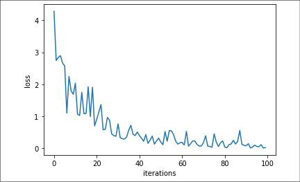
A plot, also in this case, will reveal how the optimization proceeded:

plt.plot(history)
plt.xlabel('iterations')
plt.ylabel('loss')
plt.show()

Figure 2.6: Sigmoid cross-entropy loss through iterations in our recipe

The directionality of the plot is clear, though the trajectory is a bit bumpy because we are learning one example at a time, thus making the learning process decisively stochastic. The graph could also point out the need to try to decrease the learning rate a bit.

How it works...

For a recap and explanation, for both examples, we did the following:

1. We created the data. Both examples needed to load data into specific variables used by the function that computes the network.
2. We initialized variables. We used some random Gaussian values, but initialization is a topic on its own, since much of the final results may depend on how we initialize our network (just change the random seed before initialization to find it out).
3. We created a loss function. We used the L2 loss for regression and the cross-entropy loss for classification.
4. We defined an optimization algorithm. Both algorithms used gradient descent.
5. We iterated across random data samples to iteratively update our variables.

There's more...

As we mentioned before, the optimization algorithm is sensitive to the choice of learning rate. It is important to summarize the effect of this choice in a concise manner:

Sometimes, the standard gradient descent algorithm can be stuck or slow down significantly. This can happen when the optimization is stuck in the flat spot of a saddle. To combat this, the solution is taking into account a momentum term, which adds on a fraction of the prior step's gradient descent value. You can access this solution by setting the momentum and the Nesterov parameters, along with your learning rate, in tf.optimizers.SGD (see https://www.TensorFlow.org/api_docs/python/tf/keras/optimizers/SGD for more details).

Another variant is to vary the optimizer step for each variable in our models. Ideally, we would like to take larger steps for smaller moving variables and shorter steps for faster changing variables. We will not go into the mathematics of this approach, but a common implementation of this idea is called the Adagrad algorithm. This algorithm takes into account the whole history of the variable gradients. The function in TensorFlow for this is called AdagradOptimizer() (https://www.TensorFlow.org/api_docs/python/tf/keras/optimizers/Adagrad).

Sometimes, Adagrad forces the gradients to zero too soon because it takes into account the whole history. A solution to this is to limit how many steps we use. This is called the Adadelta algorithm. We can apply this by using the AdadeltaOptimizer() function (https://www.TensorFlow.org/api_docs/python/tf/keras/optimizers/Adadelta).

There are a few other implementations of different gradient descent algorithms. For these, refer to the TensorFlow documentation at https://www.TensorFlow.org/api_docs/python/tf/keras/optimizers.

See also

For some references on optimization algorithms and learning rates, see the following papers and articles:

• Recipes from this chapter, as follows:
  • The Implementing Loss Functions section.
  • The Implementing Backpropagation section.
• Kingma, D., Jimmy, L. Adam: A Method for Stochastic Optimization. ICLR 2015 https://arxiv.org/pdf/1412.6980.pdf
• Ruder, S. An Overview of Gradient Descent Optimization Algorithms. 2016 https://arxiv.org/pdf/1609.04747v1.pdf
• Zeiler, M. ADADelta: An Adaptive Learning Rate Method. 2012 https://arxiv.org/pdf/1212.5701.pdf