Sign In Start Free Trial
Account

Add to playlist

Create a Playlist

Modal Close icon
You need to login to use this feature.
  • Book Overview & Buying Exploratory Data Analysis with Python Cookbook
  • Table Of Contents Toc
Exploratory Data Analysis with Python Cookbook

Exploratory Data Analysis with Python Cookbook

By : Ayodele Oluleye
4.8 (5)
close
close
Exploratory Data Analysis with Python Cookbook

Exploratory Data Analysis with Python Cookbook

4.8 (5)
By: Ayodele Oluleye

Overview of this book

In today's data-centric world, the ability to extract meaningful insights from vast amounts of data has become a valuable skill across industries. Exploratory Data Analysis (EDA) lies at the heart of this process, enabling us to comprehend, visualize, and derive valuable insights from various forms of data. This book is a comprehensive guide to Exploratory Data Analysis using the Python programming language. It provides practical steps needed to effectively explore, analyze, and visualize structured and unstructured data. It offers hands-on guidance and code for concepts such as generating summary statistics, analyzing single and multiple variables, visualizing data, analyzing text data, handling outliers, handling missing values and automating the EDA process. It is suited for data scientists, data analysts, researchers or curious learners looking to gain essential knowledge and practical steps for analyzing vast amounts of data to uncover insights. Python is an open-source general purpose programming language which is used widely for data science and data analysis given its simplicity and versatility. It offers several libraries which can be used to clean, analyze, and visualize data. In this book, we will explore popular Python libraries such as Pandas, Matplotlib, and Seaborn and provide workable code for analyzing data in Python using these libraries. By the end of this book, you will have gained comprehensive knowledge about EDA and mastered the powerful set of EDA techniques and tools required for analyzing both structured and unstructured data to derive valuable insights.
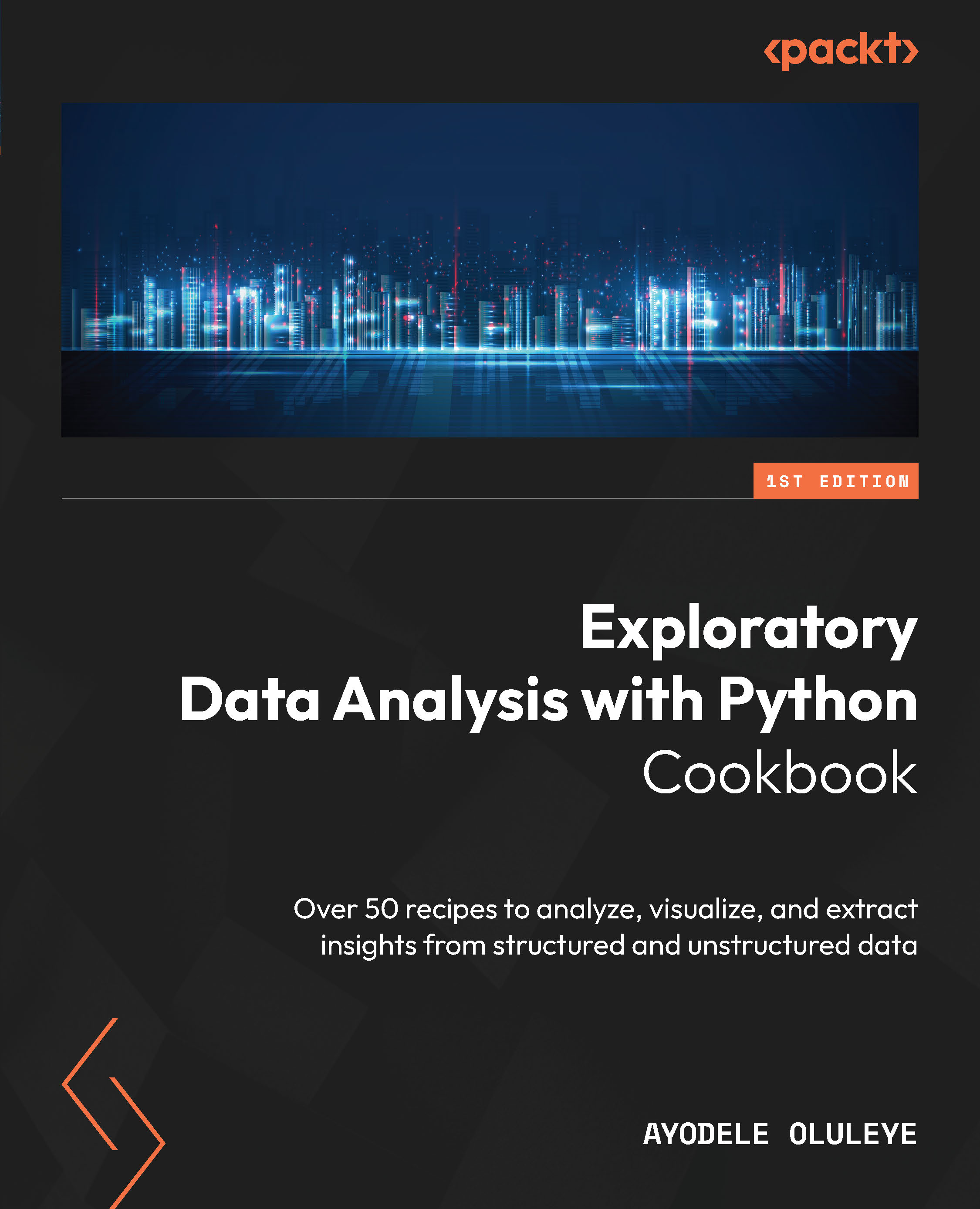
Table of Contents (13 chapters)
close
close

Categorizing data

When we refer to categorizing data, we are specifically referring to binning, bucketing, or cutting a dataset. Binning involves grouping the numeric values in a dataset into smaller intervals called bins or buckets. When we bin numerical values, each bin becomes a categorical value. Bins are very useful because they can provide us with insights that may have been difficult to spot if we had worked directly with individual numerical values. Bins don’t always have equal intervals; the creation of bins is dependent on our understanding of a dataset.

Binning can also be used to address outliers or reduce the effect of observation errors. Outliers are unusually high or unusually low data points that are far from other data points in our dataset. They typically lead to anomalies in the output of our analysis. Binning can reduce this effect by placing the range of numerical values including the outliers into specific buckets, thereby making the values categorical. A common example of this is when we convert age values into age groups. Outlier ages such as 0 or 150 can fall into a less than age 18 bin and greater than age 80 bin respectively.

In pandas, the cut method can be used to bin a dataset.

Getting ready

We will work with the full Marketing Campaign data for this recipe.

How to do it…

We will categorize data using the pandas library:

  1. Import the pandas library:
    import pandas as pd
  2. Load the .csv file into a dataframe using read_csv. Then, subset the dataframe to include only relevant columns:
    marketing_data = pd.read_csv("data/marketing_campaign.csv")
    marketing_data = marketing_data[['ID','Year_Birth', 'Education','Marital_Status','Income','Kidhome', 'Teenhome', 'Dt_Customer',              'Recency','NumStorePurchases', 'NumWebVisitsMonth']]
  3. Inspect the data. Check the first few rows and use transpose (T) to show more information. Also, check the data types as well as the number of columns and rows:
    marketing_data.head(2).T
                0    1
    ID    5524    2174
    Year_Birth    1957    1954
    Education    Graduation    Graduation
    …        …        …
    NumWebVisitsMonth    7    5
    marketing_data.dtypes
    ID    int64
    Year_Birth    int64
    Education    object
    …          …
    NumWebVisitsMonth    int64
    marketing_data.shape
    (2240, 11)
  4. Categorize the number of store purchases into high, moderate, and low categories:
    marketing_data['bins'] = pd.cut(x=marketing_data['NumStorePurchases'], bins=[0,4,8,13],labels = ['Low', 'Moderate', 'High'])
  5. Inspect the result. Subset for relevant columns:
    marketing_data[['NumStorePurchases','bins']].head()
        NumStorePurchases    bins
    0    4    Low
    1    2    Low
    2    10    High
    3    4    Low
    4    6    Moderate

We have now categorized our dataset into bins.

How it works...

We refer to pandas as pd in step 1. In step 2, we use read_csv to load the .csv file into a pandas dataframe and call it marketing_data. We also subset the dataframe to include only 11 relevant columns. In step 3, we inspect the dataset using head(2) to see the first two rows in the dataset; we also use transpose (T) along with head to transform the rows into columns due to the size of the data (i.e., it has many columns). We use the dtypes attribute of the dataframe to show the data types of all columns. Numeric data has int and float data types while character data has the object data type. We inspect the number of rows and columns using shape, which returns a tuple that displays the number of rows and columns respectively.

In step 4, we categorize the number of store purchases into three categories, namely High, Moderate, and Low. Using the cut method, we cut NumStorePurchases into these three bins and supply the logic for binning within the bin parameter, which is the second parameter. The third parameter is the label parameter. Whenever we manually supply the bin edges in a list as done previously, the bins are typically the number of label categories + 1.

Our bins can be interpreted as 0–4 (low), 5–8 (moderate), and 9–13 (high). In step 5, we subset for relevant columns and inspect the result of our binning.

There’s more...

For the bin argument, we can also supply the number of bins we require instead of supplying the bin edges manually. This means in the previous steps, we could have supplied the value 3 to the bin parameter and the cut method would have categorized our data into three equally spaced bins. When the value 3 is supplied, the cut method focuses on the equal spacing of the bins, even though the number of records in the bins may be different.

If we are also interested in the distribution of our bins and not just equally spaced bins or user-defined bins, the qcut method in pandas can be used. The qcut method ensures the distribution of data in the bins is equal. It ensures all bins have (roughly) the same number of observations, even though the bin range may vary.

CONTINUE READING
83
Tech Concepts
36
Programming languages
73
Tech Tools
Icon Unlimited access to the largest independent learning library in tech of over 8,000 expert-authored tech books and videos.
Icon Innovative learning tools, including AI book assistants, code context explainers, and text-to-speech.
Icon 50+ new titles added per month and exclusive early access to books as they are being written.
Exploratory Data Analysis with Python Cookbook
notes
bookmark Notes and Bookmarks search Search in title playlist Add to playlist download Download options font-size Font size

Change the font size

margin-width Margin width

Change margin width

day-mode Day/Sepia/Night Modes

Change background colour

Close icon Search
Country selected

Close icon Your notes and bookmarks

Confirmation

Modal Close icon
claim successful

Buy this book with your credits?

Modal Close icon
Are you sure you want to buy this book with one of your credits?
Close
YES, BUY

Submit Your Feedback

Modal Close icon
Modal Close icon
Modal Close icon